The metafor Package

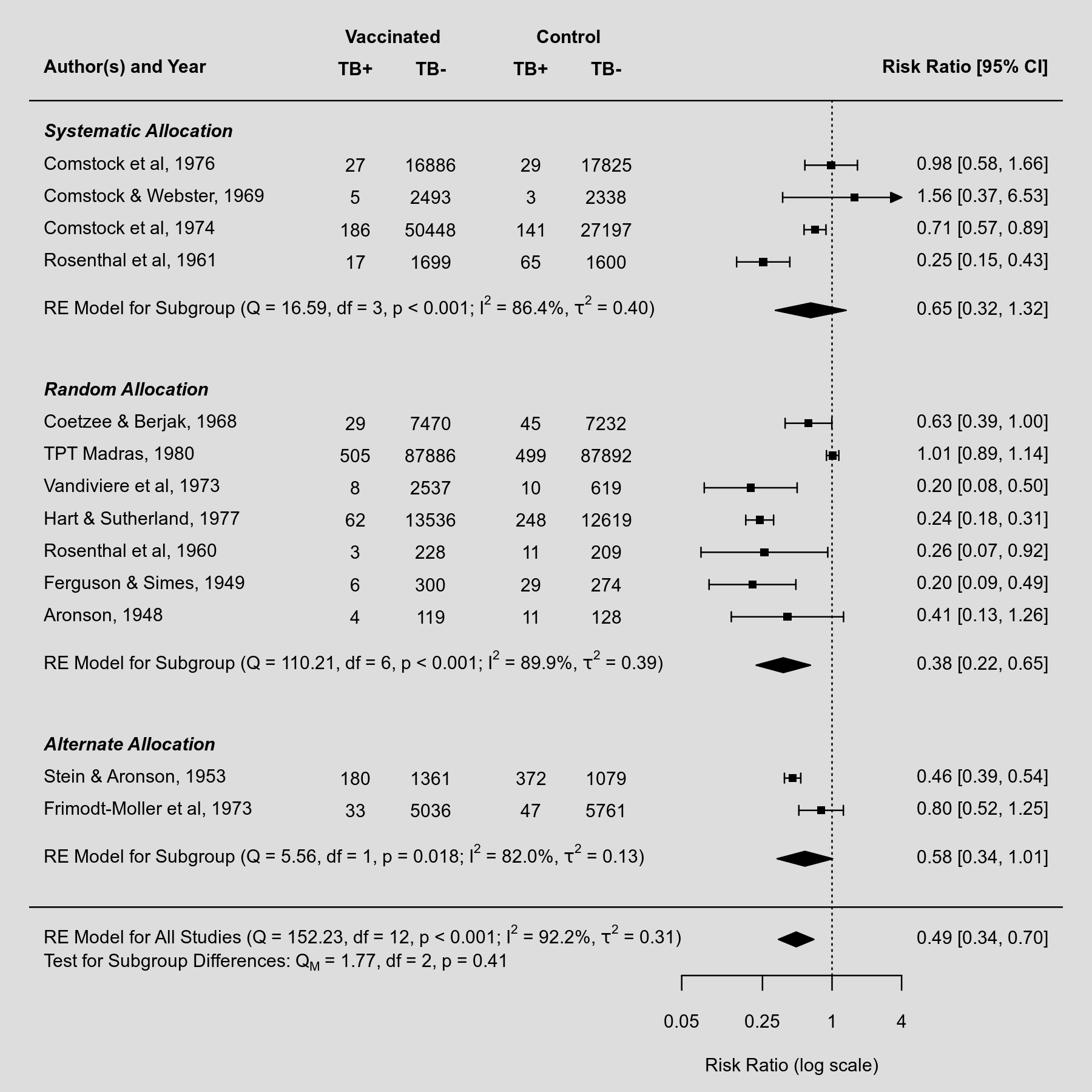
Below is an example of a forest plot with three subgroups. The results of the individual studies are shown grouped together according to their subgroup. Below each subgroup, a summary polygon shows the results when fitting a random-effects model just to the studies within that group. The summary polygon at the bottom of the plot shows the results from a random-effects model when analyzing all 13 studies.

library(metafor)
 
### copy BCG vaccine meta-analysis data into 'dat'
dat <- dat.bcg
 
### calculate log risk ratios and corresponding sampling variances (and use
### the 'slab' argument to store study labels as part of the data frame)
dat <- escalc(measure="RR", ai=tpos, bi=tneg, ci=cpos, di=cneg, data=dat,
              slab=paste(author, year, sep=", "))
 
### fit random-effects model
res <- rma(yi, vi, data=dat)
 
### a little helper function to add Q-test, I^2, and tau^2 estimate info
mlabfun <- function(text, x) {
   list(bquote(paste(.(text),
      " (Q = ", .(fmtx(x$QE, digits=2)),
      ", df = ", .(x$k - x$p), ", ",
      .(fmtp2(x$QEp)), "; ",
      I^2, " = ", .(fmtx(x$I2, digits=1)), "%, ",
      tau^2, " = ", .(fmtx(x$tau2, digits=2)), ")")))}
 
### set up forest plot (with 2x2 table counts added; the 'rows' argument is
### used to specify in which rows the outcomes will be plotted)
forest(res, xlim=c(-16, 4.6), at=log(c(0.05, 0.25, 1, 4)), atransf=exp,
       ilab=cbind(tpos, tneg, cpos, cneg), ilab.lab=c("TB+","TB-","TB+","TB-"),
       ilab.xpos=c(-9.5,-8,-6,-4.5), cex=0.75, ylim=c(-2,28), top=4, order=alloc,
       rows=c(3:4,9:15,20:23), mlab=mlabfun("RE Model for All Studies", res),
       psize=1, header="Author(s) and Year")
 
### set font expansion factor (as in forest() above)
op <- par(cex=0.75)
 
### add additional column headings to the plot
text(c(-8.75,-5.25), 27, c("Vaccinated", "Control"), font=2)
 
### add text for the subgroups
text(-16, c(24,16,5), pos=4, c("Systematic Allocation",
                               "Random Allocation",
                               "Alternate Allocation"), font=4)
 
### set par back to the original settings
par(op)
 
### fit random-effects model in the three subgroups
res.s <- rma(yi, vi, subset=(alloc=="systematic"), data=dat)
res.r <- rma(yi, vi, subset=(alloc=="random"),     data=dat)
res.a <- rma(yi, vi, subset=(alloc=="alternate"),  data=dat)
 
### add summary polygons for the three subgroups
addpoly(res.s, row=18.5, mlab=mlabfun("RE Model for Subgroup", res.s))
addpoly(res.r, row= 7.5, mlab=mlabfun("RE Model for Subgroup", res.r))
addpoly(res.a, row= 1.5, mlab=mlabfun("RE Model for Subgroup", res.a))
 
### fit meta-regression model to test for subgroup differences
res <- rma(yi, vi, mods = ~ alloc, data=dat)
 
### add text for the test of subgroup differences
text(-16, -1.8, pos=4, cex=0.75, bquote(paste("Test for Subgroup Differences: ",
     Q[M], " = ", .(fmtx(res$QM, digits=2)),
     ", df = ", .(res$p - 1), ", ", .(fmtp2(res$QMp)))))