The metafor Package

In the simplest case of a meta-analysis, each study provides a single (effect size) estimate to the analysis. A standard forest plot then shows the estimates of the studies (with corresponding confidence intervals) and the summary estimate based on the meta-analysis at the bottom of the figure. See here for an example.

However, in practice, one often encounters more complex data structures, for example where at least some of the studies contribute multiple (dependent) estimates to the analysis. Such meta-analyses also tend to involve a larger number of estimates, so that a forest plot showing all of the individual estimates from each of the studies requires a rather large figure where the size of the elements becomes quite small.

Consider the following example:

dat <- dat.assink2016
 
### turn 'dat' into an 'escalc' object (and add study labels)
dat <- escalc(measure="SMD", yi=yi, vi=vi, data=dat, slab=paste("Study", study, " Estimate", esid))
 
### assume that the effect sizes within studies are correlated with rho=0.6
V <- vcalc(vi, cluster=study, obs=esid, data=dat, rho=0.6)
 
### fit multilevel model using this approximate V matrix
res <- rma.mv(yi, V, random = ~ 1 | study/esid, data=dat, digits=3)
res

Multivariate Meta-Analysis Model (k = 100; method: REML)
 
Variance Components:
 
           estim   sqrt  nlvls  fixed      factor
sigma^2.1  0.081  0.284     17     no       study
sigma^2.2  0.155  0.393    100     no  study/esid
 
Test for Heterogeneity:
Q(df = 99) = 745.438, p-val < .001
 
Model Results:
 
estimate     se   zval   pval  ci.lb  ci.ub
   0.368  0.097  3.810  <.001  0.179  0.557  ***
 
---
Signif. codes:  0 '***' 0.001 '**' 0.01 '*' 0.05 '.' 0.1 ' ' 1

This example dataset involves 17 studies that contribute between 1 and 22 estimates to the analysis (for a total of $k = 100$ estimates). Multiple estimates arising from the same study are likely to be dependent, which was accounted for by letting the sampling errors within studies be correlated with a correlation coefficient of 0.6 and by using a multilevel model with random effects at the study and at the estimate level.¹⁾

Now we could draw a forest plot of the individual estimates as follows:

par(tck=-.01, mgp=c(1,0.01,0), mar=c(2,4,0,2))
 
dd <- c(0,diff(dat$study))
rows <- (1:res$k) + cumsum(dd)
forest(res, rows=rows, ylim=c(2,max(rows)+3), xlim=c(-5,7), cex=0.4,
       efac=c(0,1), header=TRUE, mlab="Pooled Estimate")
abline(h = rows[c(1,diff(rows)) == 2] - 1, lty="dotted")

Note that by making some clever use of the rows argument, we can even group the estimates of studies together and differentiate different studies with horizontal dotted lines. The resulting forest plot looks like this:

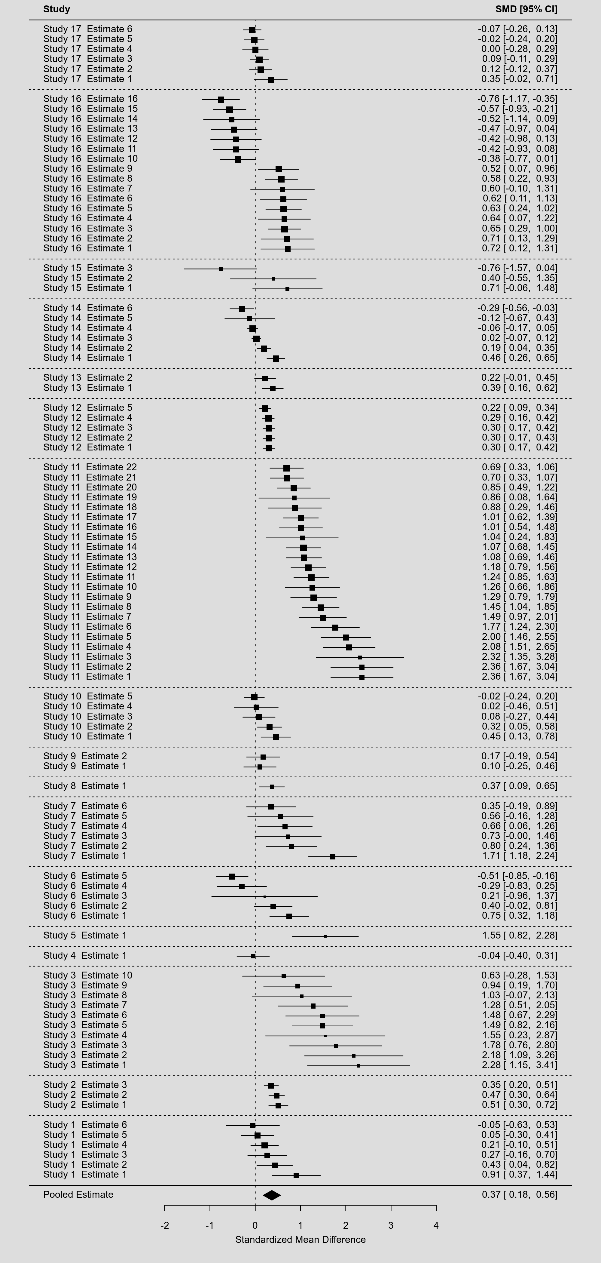
By squeezing so many estimates into a single figure, the various elements in the plot become so small that they are hardly legible. As an alternative, we could consider not showing the individual estimates, but pooled estimates that are aggregated to the study level. To do such within-study averaging properly, we need to extract the marginal variance-covariance matrix of the estimates based on the multilevel model and use this in combination with the aggregate() function as follows (keeping only the variables needed):

agg <- aggregate(dat, cluster=study, V=vcov(res, type="obs"), addk=TRUE)
agg <- agg[c(1,4,5,9)]
agg

   study      yi     vi ki
1      1  0.2865 0.1371  6
2      2  0.4457 0.1384  3
3      3  1.2533 0.2145 10
4      4 -0.0447 0.2684  1
5      5  1.5490 0.3737  1
6      6  0.0844 0.1527  5
7      7  0.8452 0.1693  6
8      8  0.3695 0.2552  1
9      9  0.1396 0.1851  2
10    10  0.1765 0.1302  5
11    11  1.0536 0.1178 22
12    12  0.2811 0.1145  5
13    13  0.3026 0.1690  2
14    14  0.0518 0.1143  6
15    15  0.1010 0.2641  3
16    16  0.0775 0.1240 16
17    17  0.0683 0.1172  6

When aggregating the estimates in this manner, it turns out that a meta-analysis of these pooled estimates yields exactly the same results as those obtained from the multilevel model above:

res <- rma(yi, vi, method="EE", data=agg, digits=3)
res

Model Results:
 
estimate     se   zval   pval  ci.lb  ci.ub
   0.368  0.097  3.810  <.001  0.179  0.557  ***

Note that an equal-effects model is used above, since the heterogeneity (at the study and effect size levels) was already accounted for in the aggregation step (via the marginal variance-covariance matrix of the estimates extracted from the model). Also, the rest of the output, such as the $I^2$ value and the results from the $Q$-test, should be ignored and hence are not shown above.

We can now draw a forest plot based on the aggregated estimates (including again the pooled estimate from the model) as follows:

forest(res, xlim=c(-4,5), mlab="Pooled Estimate", header=TRUE, ilab=ki, ilab.xpos=-2)
text(-2, res$k+2, "Estimates", font=2)

This figure would be much easier to include in a paper or presentation (with a footnote that it shows the aggregated estimates, but that the actual analysis was conducted based on the $k=100$ individual estimates using a multilevel model).

A final note: Within-study averaging has often been used in the past as a method for avoiding dependent estimates, so that the actual analysis could be conducted with simpler methods. However, this is no longer necessary, as we have methods and software now for conducting multivariate/multilevel analyses that can account for dependent estimates. Moreover, the way such averaging has often been done in the past involves various simplifying (and often untenable) assumptions that should no longer be used in practice. Note that we actually had to fit the multilevel model above in order to aggregate the estimates to the study level in such a way that the results from a pooled analysis of these aggregated estimates are identical to those from the multilevel model. This would not be the case when using simpler methods for doing the within-study averaging.