Table of Contents
Yusuf et al. (1985)
The Methods and Data
The meta-analysis by Yusuf et al. (1985) on the effectiveness of beta blockers for reducing mortality and reinfarction is usually cited as the reference for what is sometimes called Peto's (one-step or modified Mantel-Haenszel) method for meta-analyzing 2×2 table data. The method provides a weighted estimate of the (log) odds ratio under an equal-effects model and is particularly advantageous when the event of interest is rare. However, it should only be used when the group sizes within the individual studies are not too dissimilar and effect sizes are generally small (Greenland & Salvan, 1990; Sweeting et al., 2004; Bradburn et al., 2007). This method is implemented in the rma.peto() function and can be illustrated with this dataset.
The data can be loaded with:
library(metafor)
dat <- dat.yusuf1985
dat$grp_ratios <- round(dat$n1i / dat$n2i, 2)
(I copy the dataset into dat, which is a bit shorter and therefore easier to type further below). The last command adds the ratio of the group sizes as a variable to the data frame. This will be useful for checking on strong imbalances in group sizes. Note that the dataset actually includes the data from multiple tables. Table 6 (p. 343) from the article includes the results from short-term trials of oral beta blockers:
dat[dat$table=="6",]
   table   id       trial ai n1i ci n2i grp_ratios
1      6  1.1      Balcon 14  56 15  58       0.97
2      6  1.2     Clausen 18  66 19  64       1.03
3      6  1.3 Multicentre 15 100 12  95       1.05
4      6  1.4      Barber 10  52 12  47       1.11
5      6  1.5      Norris 21 226 24 228       0.99
6      6  1.6      Kahler  3  38  6  31       1.23
7      6  1.7     Ledwich  2  20  3  20       1.00
8      6  1.8      Snow 1 NA  NA NA  NA         NA
9      6  1.9      Snow 2 19  76 15  67       1.13
10     6 1.10    Fuccella 15 106  9 114       0.93
11     6 1.11      Briant  5  62  4  57       1.09
12     6 1.12        Pitt  0   9  0   8       1.12
13     6 1.13    Lombardo  8 133 11 127       1.05
14     6 1.14    Thompson  3  48  3  49       0.98
15     6 1.15      Hutton  0  16  0  13       1.23
16     6 1.16      Tonkin  1  42  1  46       0.91
17     6 1.17       Gupta  0  25  3  25       1.00
18     6  2.1      Barber 14 221 15 228       0.97
19     6  2.2       Yusuf  0  11  0  11       1.00
20     6  2.3    Wilcox 1  8 259  7 129       2.01
21     6  2.4    Wilcox 2  6 157  4 158       0.99
22     6  2.5        CPRG  3 177  2 136       1.30
Data Checks
As can been seen from the output above, the great majority of the studies in Table 6 are quite balanced. To check that the individual effect sizes are generally not too large, we can create a likelihood plot for the odds ratios in the individual studies with:
par(mfrow=c(1,2))
llplot(measure="OR", ai=ai, n1i=n1i, ci=ci, n2i=n2i, data=dat,
       subset=(table=="6"), drop00=FALSE, lwd=1, xlim=c(-5,5))
llplot(measure="OR", ai=ai, n1i=n1i, ci=ci, n2i=n2i, data=dat,
       subset=(table=="6"), drop00=FALSE, lwd=1, xlim=c(-5,5), scale=FALSE)
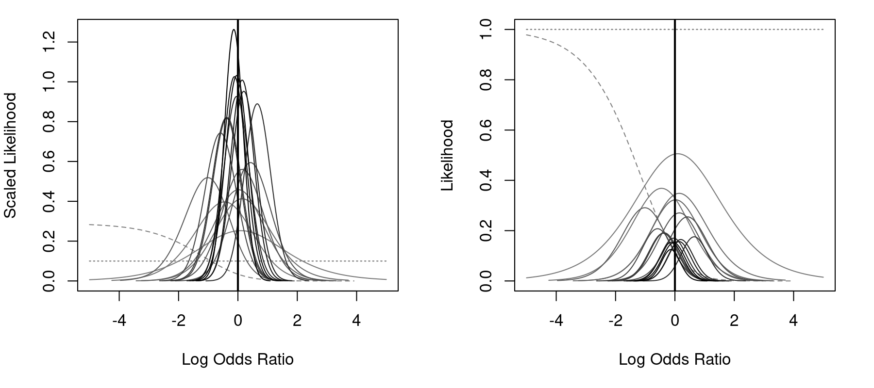
The left figure uses scaling (by default), so that the total area under each curve is (approximately) equal to 1, while the right figure does not use scaling. Three studies actually had no events in either group. For these studies, the likelihood is flat, as indicated by the horizontal dotted lines (by default, these studies would have been automatically omitted from the plot; by setting drop00=FALSE, they are shown). Finally, one study had zero events in the treatment group, but 3 events in the control group. For this study, the MLE of the odds ratio is negative infinity. The dashed line corresponds to the likelihood for this study. However, for the great majority of the studies, the peak of the likelihoods is close to 0 (i.e., an odds ratio of 1)
Analysis of Table 6
We can now proceed with the analysis of the data in Table 6 using Peto's method:
res <- rma.peto(ai=ai, n1i=n1i, ci=ci, n2i=n2i,
                data=dat, subset=(table=="6"))
res
Equal-Effects Model (k = 21)

I^2 (total heterogeneity / total variability):  0.00%
H^2 (total variability / sampling variability): 0.64

Test for Heterogeneity:
Q(df = 17) = 10.8275, p-val = 0.8654

Model Results (log scale):

estimate      se     zval    pval    ci.lb   ci.ub
 -0.0692  0.1194  -0.5794  0.5623  -0.3031  0.1648

Model Results (OR scale):

estimate   ci.lb   ci.ub
  0.9332  0.7385  1.1792
Or, to round the estimated odds ratio to 2 digits, we can use:
predict(res, transf=exp, digits=2)
 pred ci.lb ci.ub
 0.93  0.74  1.18
These results match what is reported underneath Table 6 (p. 343).
Analysis via the Inverse-Variance Method
Peto's method actually is equivalent to using a standard (inverse-variance) equal-effects model approach, but estimating the (log) odds ratio and corresponding sampling variance within each study based on the efficient score and Fisher's information evaluated at $\theta_i = 0$ (where $\theta_i$ is the true log odds ratio). We can do this explicitly with:
dat <- escalc(measure="PETO", ai=ai, n1i=n1i, ci=ci, n2i=n2i,
              data=dat, subset=(table=="6"), add=0)
dat
   table   id       trial ai n1i ci n2i grp_ratios      yi     vi
1      6  1.1      Balcon 14  56 15  58       0.97 -0.0451 0.1834
2      6  1.2     Clausen 18  66 19  64       1.03 -0.1177 0.1500
3      6  1.3 Multicentre 15 100 12  95       1.05  0.1975 0.1712
4      6  1.4      Barber 10  52 12  47       1.11 -0.3609 0.2320
5      6  1.5      Norris 21 226 24 228       0.99 -0.1379 0.0985
6      6  1.6      Kahler  3  38  6  31       1.23 -0.9958 0.5089
7      6  1.7     Ledwich  2  20  3  20       1.00 -0.4457 0.8914
8      6  1.8      Snow 1 NA  NA NA  NA         NA      NA     NA
9      6  1.9      Snow 2 19  76 15  67       1.13  0.1431 0.1539
10     6 1.10    Fuccella 15 106  9 114       0.93  0.6408 0.1865
11     6 1.11      Briant  5  62  4  57       1.09  0.1485 0.4776
12     6 1.12        Pitt  0   9  0   8       1.12      NA     NA
13     6 1.13    Lombardo  8 133 11 127       1.05 -0.3892 0.2264
14     6 1.14    Thompson  3  48  3  49       0.98  0.0218 0.7034
15     6 1.15      Hutton  0  16  0  13       1.23      NA     NA
16     6 1.16      Tonkin  1  42  1  46       0.91  0.0922 2.0274
17     6 1.17       Gupta  0  25  3  25       1.00 -2.0851 1.3901
18     6  2.1      Barber 14 221 15 228       0.97 -0.0403 0.1472
19     6  2.2       Yusuf  0  11  0  11       1.00      NA     NA
20     6  2.3    Wilcox 1  8 259  7 129       2.01 -0.6273 0.3117
21     6  2.4    Wilcox 2  6 157  4 158       0.99  0.4183 0.4118
22     6  2.5        CPRG  3 177  2 136       1.30  0.1423 0.8245
Note that with add=0, no adjustments to the observed counts are made, so that studies with zero events are essentially dropped from further analyses.
Now, an equal-effects model using the standard (inverse-variance) approach can be fitted with:
res <- rma(yi, vi, data=dat, method="EE")
res
Equal-Effects Model (k = 18)

I^2 (total heterogeneity / total variability):   0.00%
H^2 (total variability / sampling variability):  0.64

Test for Heterogeneity:
Q(df = 17) = 10.8275, p-val = 0.8654

Model Results:

estimate      se     zval    pval    ci.lb   ci.ub
 -0.0692  0.1194  -0.5794  0.5623  -0.3031  0.1648

---
Signif. codes:  0 '***' 0.001 '**' 0.01 '*' 0.05 '.' 0.1 ' ' 1
The estimated log odds ratio can be back-transformed through exponentiation:
predict(res, transf=exp, digits=2)
 pred ci.lb ci.ub
 0.93  0.74  1.18
Note that these are exactly the same results as obtained earlier.
The remaining tables (i.e., 9, 10, 11, 12a, and 12b) can be analyzed accordingly.
References
Bradburn, M. J., Deeks, J. J., Berlin, J. A., & Localio, A. R. (2007). Much ado about nothing: A comparison of the performance of meta-analytical methods with rare events. Statistics in Medicine, 26(1), 53–77.
Greenland, S., & Salvan, A. (1990). Bias in the one-step method for pooling study results. Statistics in Medicine, 9(3), 247–252.
Sweeting, M. J., Sutton, A. J., & Lambert, P. C. (2004). What to add to nothing? Use and avoidance of continuity corrections in meta-analysis of sparse data. Statistics in Medicine, 23(9), 1351–1375.
Yusuf, S., Peto, R., Lewis, J., Collins, R., & Sleight, P. (1985). Beta blockade during and after myocardial infarction: An overview of the randomized trials. Progress in Cardiovascular Disease, 27(5), 335–371.