The metafor Package

Viechtbauer (2007) describes various methods for computing confidence intervals (CIs) for the amount of heterogeneity in random-effects models. An example dataset, based on a meta-analysis by Collins et al. (1985) examining the effectiveness of diuretics in pregnancy for preventing pre-eclampsia, is used in the paper to illustrate the various methods. The data are given in the paper in Table I (p. 44).

The data can be loaded with:

library(metafor)
dat <- dat.collins1985b[,1:7]
dat

We only need the first 7 columns of the dataset (the remaining columns pertain to other outcomes). The contents of the dataset are:

  id                  author year pre.nti pre.nci pre.xti pre.xci
1  1       Weseley & Douglas 1962     131     136      14      14
2  2          Flowers et al. 1962     385     134      21      17
3  3                 Menzies 1964      57      48      14      24
4  4           Fallis et al. 1964      38      40       6      18
5  5         Cuadros & Tatum 1964    1011     760      12      35
6  6        Landesman et al. 1965    1370    1336     138     175
7  7            Kraus et al. 1966     506     524      15      20
8  8    Tervila & Vartiainen 1971     108     103       6       2
9  9 Campbell & MacGillivray 1975     153     102      65      40

Variables pre.nti and pre.nci indicate the number of women in the treatment and control/placebo groups, respectively, while pre.xti and pre.xci indicate the number of women in the respective groups with any form of pre-eclampsia during the pregnancy.

The corresponding log odds ratios (and corresponding sampling variances) can then be computed and added to the dataset with:

dat <- escalc(measure="OR", ai=pre.xti, n1i=pre.nti, ci=pre.xci, n2i=pre.nci, data=dat)
dat

  id                  author year pre.nti pre.nci pre.xti pre.xci      yi     vi
1  1       Weseley & Douglas 1962     131     136      14      14  0.0418 0.1596
2  2          Flowers et al. 1962     385     134      21      17 -0.9237 0.1177
3  3                 Menzies 1964      57      48      14      24 -1.1221 0.1780
4  4           Fallis et al. 1964      38      40       6      18 -1.4733 0.2989
5  5         Cuadros & Tatum 1964    1011     760      12      35 -1.3910 0.1143
6  6        Landesman et al. 1965    1370    1336     138     175 -0.2969 0.0146
7  7            Kraus et al. 1966     506     524      15      20 -0.2615 0.1207
8  8    Tervila & Vartiainen 1971     108     103       6       2  1.0888 0.6864
9  9 Campbell & MacGillivray 1975     153     102      65      40  0.1353 0.0679

We can obtain the various estimates of the amount of heterogeneity (i.e., $\tau^2$) with:

res.DL   <- rma(yi, vi, data=dat, method="DL")
res.ML   <- rma(yi, vi, data=dat, method="ML")
res.REML <- rma(yi, vi, data=dat, method="REML")
res.SJ   <- rma(yi, vi, data=dat, method="SJ")
round(c(DL=res.DL$tau2, ML=res.ML$tau2, REML=res.REML$tau2, SJ=res.SJ$tau2), 2)

  DL   ML REML   SJ
0.23 0.24 0.30 0.46

These are the same values as given in Table II (p. 44) of the paper (the Sidik–Jonkman estimator is denoted as $\hat{\tau}^2_{SH}$ in the paper).

Next, we will obtain the various CIs for $\tau^2$, also as given in the paper in Table II.

First, the Q-profile CI can be obtained with:

confint(res.DL, digits=2)

       estimate ci.lb ci.ub
tau^2      0.23  0.07  2.20
tau        0.48  0.27  1.48
I^2(%)    70.66 43.12 95.85
H^2        3.41  1.76 24.09

Note that CIs for the $I^2$ and $H^2$ statistics are also provided.

The following code can be used to obtain the CI based on the method by Biggerstaff and Tweedie (1997):

CI.D.func <- function(tau2val, s1, s2, Q, k, lower.tail) {
   expQ  <- (k-1) + s1*tau2val
   varQ  <- 2*(k-1) + 4*s1*tau2val + 2*s2*tau2val^2
   shape <- expQ^2/varQ
   scale <- varQ/expQ
   qtry  <- Q/scale
   pgamma(qtry, shape = shape, scale = 1, lower.tail = lower.tail) - 0.025
}
 
wi <- 1/dat$vi
s1 <- sum(wi) - sum(wi^2)/sum(wi)
s2 <- sum(wi^2) - 2*sum(wi^3)/sum(wi) + sum(wi^2)^2/sum(wi)^2
 
ci.lb <- uniroot(CI.D.func, interval=c(0,10), s1=s1, s2=s2,
                 Q=res.DL$QE, k=res.DL$k, lower.tail=FALSE)$root
ci.ub <- uniroot(CI.D.func, interval=c(0,10), s1=s1, s2=s2,
                 Q=res.DL$QE, k=res.DL$k, lower.tail=TRUE)$root
round(c(ci.lb=ci.lb, ci.ub=ci.ub), 2)

ci.lb ci.ub
 0.05  2.36

Profile likelihood methods for meta-analysis were described by Hardy and Thompson (1996). By setting type="PL", we can obtain the profile likelihood CI for $\tau^2$ with:

confint(res.ML, type="PL", digits=2)

       estimate ci.lb ci.ub
tau^2      0.24  0.03  1.13
tau        0.49  0.16  1.06
I^2(%)    71.44 21.78 92.22
H^2        3.50  1.28 12.85

With the code below, we can obtain a plot of the profile log-likelihood as a function of $\tau^2$:

profile(res.ML, xlim=c(0,1.2), steps=50, cline=TRUE)
tmp <- confint(res.ML, type="PL", digits=2)
abline(v=tmp$random[1, 2:3], lty="dotted")

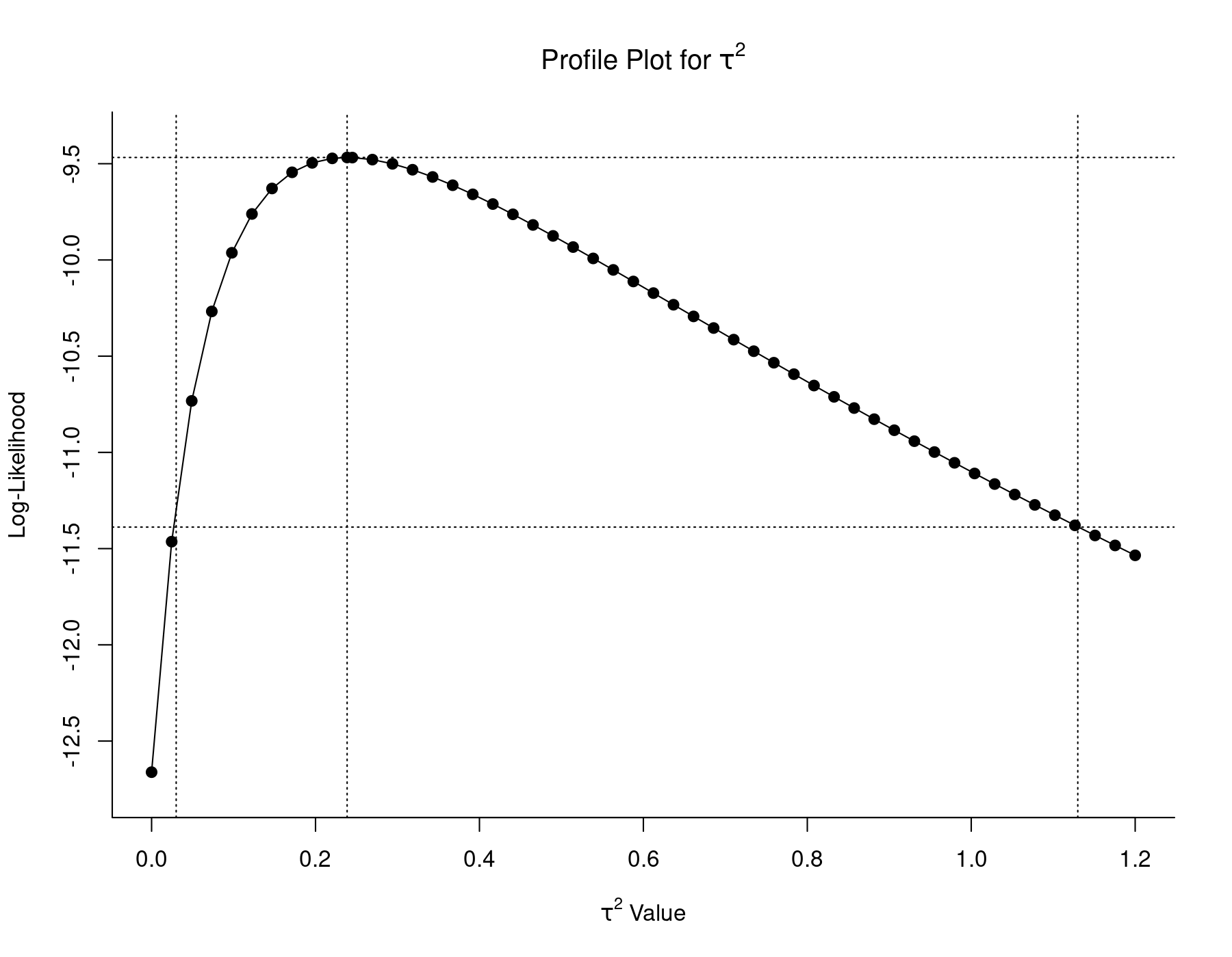
The middle vertical line indicates the ML estimate of $\tau^2$, with the upper horizontal line denoting the corresponding log-likelihood. The lower horizontal line corresponds to this log-likelihood value minus 3.84/2. Therefore, the two $\tau^2$ values with log-likelihoods equal to this value are the bounds of a 95% profile likelihood CI for $\tau^2$. These values are approximately equal to 0.03 and 1.13, as indicated by the left and right vertical lines.

A profile likelihood CI for $\tau^2$ can also be obtained based on REML estimation:

confint(res.REML, type="PL", digits=2)

       estimate ci.lb ci.ub
tau^2      0.30  0.04  1.47
tau        0.55  0.21  1.21
I^2(%)    75.92 30.94 93.92
H^2        4.15  1.45 16.46

The plot of the restricted log-likelihood can again be obtained with:

profile(res.REML, xlim=c(0,1.6), steps=50, cline=TRUE)
tmp <- confint(res.REML, type="PL", digits=2)
abline(v=tmp$random[1, 2:3], lty="dotted")

Based on the restricted log-likelihood function, the bounds of the 95% profile likelihood CI are approximately equal to 0.04 and 1.47.

Note: When using the rma.mv() function for the model fitting, confint() directly provides profile likelihood CIs (see here for a comparison of the rma() and rma.mv() functions). The syntax is then:

res <- rma.mv(yi, vi, random = ~ 1 | id, data=dat, method="ML")
confint(res, digits=2)

        estimate ci.lb ci.ub
sigma^2     0.24  0.03  1.13
sigma       0.49  0.16  1.06

res <- rma.mv(yi, vi, random = ~ 1 | id, data=dat, method="REML")
confint(res, digits=2)

        estimate ci.lb ci.ub
sigma^2     0.30  0.04  1.47
sigma       0.55  0.21  1.21

Note that the variance component is called sigma^2 here. The CI bounds match those described above.

The Wald-type CIs based on ML and REML estimation can be obtained with:

round(c(ci.lb=res.ML$tau2 - 1.96*res.ML$se.tau2,
        ci.ub=res.ML$tau2 + 1.96*res.ML$se.tau2), 2)

ci.lb ci.ub
-0.10  0.58

and

round(c(ci.lb=res.REML$tau2 - 1.96*res.REML$se.tau2,
        ci.ub=res.REML$tau2 + 1.96*res.REML$se.tau2), 2)

ci.lb ci.ub
-0.13  0.73

The lower bounds of the CIs fall below 0 and could be truncated to zero (to avoid values outside of the parameter space). However, Wald-type CIs for variance components should best be avoided in the first place (since the normal distribution typically provides a poor approximation to the distribution of ML and REML estimates of variance components).

Together with their estimator, Sidik and Jonkman (2005) described a simple method for obtaining a confidence interval for $\tau^2$. The CI can be obtained with:

round(c(ci.lb=(res.SJ$k-1) * res.SJ$tau2 / qchisq(0.975, df=res.SJ$k-1),
        ci.ub=(res.SJ$k-1) * res.SJ$tau2 / qchisq(0.025, df=res.SJ$k-1)), 2)

ci.lb ci.ub
 0.21  1.67

The boot package can be used obtain the parametric and non-parametric bootstrap CIs, so let's load the package first:

library(boot)

For parametric bootstrapping, we need to define two functions, one for calculating the statistic of interest (and possibly its variance) based on the bootstrap data, the second for actually generating the bootstrap data.

boot.func <- function(data.boot) {
   res <- rma(yi, vi, data=data.boot, method="DL")
   c(res$tau2, res$se.tau2^2)
}
 
data.gen <- function(dat, mle) {
   data.frame(yi=rnorm(nrow(dat), mle$mu, sqrt(mle$tau2 + dat$vi)), vi=dat$vi)
}

Next, we can do the bootstrapping (based on 1000 bootstrap samples) and then obtain a variety of different bootstrap CIs:

sav <- boot(dat, boot.func, R=1000, sim="parametric", ran.gen=data.gen,
            mle=list(mu=coef(res.DL), tau2=res.DL$tau2))
boot.ci(sav, type=c("norm", "basic", "stud", "perc"))

BOOTSTRAP CONFIDENCE INTERVAL CALCULATIONS
Based on 1000 bootstrap replicates
 
CALL :
boot.ci(boot.out = sav, type = c("norm", "basic", "stud", "perc"))
 
Intervals :
Level      Normal              Basic
95%   (-0.1298,  0.5907 )   (-0.2535,  0.4594 )
 
Level    Studentized          Percentile
95%   ( 0.0508,  1.1814 )   ( 0.0000,  0.7129 )
Calculations and Intervals on Original Scale

In the paper, the percentile CI is reported (untruncated, so the lower bound actually falls below 0). The upper bound is slightly different than the one shown above due to the random play of chance when bootstrapping with a finite number of samples.

For the non-parametric bootstrap method, we only need to define one function with two arguments, one for the original data and one for a vector of indices which define the bootstrap sample. The function again returns the statistic of interest (and its variance):

boot.func <- function(dat, indices) {
   res <- rma(yi, vi, data=dat, subset=indices, method="DL")
   c(res$tau2, res$se.tau2^2)
}

It then takes again two lines of code to conduct the actual boostrapping and obtain the corresponding CIs:

sav <- boot(dat, boot.func, R=1000)
boot.ci(sav)

BOOTSTRAP CONFIDENCE INTERVAL CALCULATIONS
Based on 1000 bootstrap replicates
 
CALL :
boot.ci(boot.out = sav)
 
Intervals :
Level      Normal              Basic             Studentized
95%   (-0.0178,  0.4953 )   (-0.0517,  0.4372 )   ( 0.0789,  1.1202 )
 
Level     Percentile            BCa
95%   ( 0.0222,  0.5111 )   ( 0.0361,  0.5641 )
Calculations and Intervals on Original Scale

Again, the percentile CI is reported in the paper, with the small difference resulting from the play of chance. For more details on bootstrapping, see bootstrapping with meta-analytic models under the tips and notes section.

Biggerstaff, B. J., & Tweedie, R. L. (1997). Incorporating variability in estimates of heterogeneity in the random effects model in meta-analysis. Statistics in Medicine, 16(7), 753–768.

Hardy, R. J., & Thompson, S. G. (1996). A likelihood approach to meta-analysis with random effects. Statistics in Medicine, 15(6), 619–629.

Sidik, K., & Jonkman, J. N. (2005). Simple heterogeneity variance estimation for meta-analysis. Applied Statistics, 54(2), 367–384.

Viechtbauer, W. (2007). Confidence intervals for the amount of heterogeneity in meta-analysis. Statistics in Medicine, 26(1), 37–52.