Forest Plot with Exact Confidence Intervals
A forest plot is a commonly used visualization technique in meta-analyses, showing the results of the individual studies (i.e., the estimated effects or observed outcomes) together with their (usually 95%) confidence intervals (CIs). A four-sided polygon, sometimes called a summary 'diamond', is added to the bottom of the plot, showing the summary estimate based on the model (with the center of the polygon corresponding to the estimate and the left/right edges indicating the confidence interval limits).
Let's create such a figure for our beloved BCG vaccine dataset. First, we compute the log odds ratios and corresponding sampling variances for the studies with:
dat <- dat.bcg
dat <- escalc(measure="OR", ai=tpos, bi=tneg, ci=cpos, di=cneg, data=dat,
              slab=paste(author, year, sep=", "))
dat
   trial               author year tpos  tneg cpos  cneg ablat      alloc      yi     vi
1      1              Aronson 1948    4   119   11   128    44     random -0.9387 0.3571
2      2     Ferguson & Simes 1949    6   300   29   274    55     random -1.6662 0.2081
3      3      Rosenthal et al 1960    3   228   11   209    42     random -1.3863 0.4334
4      4    Hart & Sutherland 1977   62 13536  248 12619    52     random -1.4564 0.0203
5      5 Frimodt-Moller et al 1973   33  5036   47  5761    13  alternate -0.2191 0.0520
6      6      Stein & Aronson 1953  180  1361  372  1079    44  alternate -0.9581 0.0099
7      7     Vandiviere et al 1973    8  2537   10   619    19     random -1.6338 0.2270
8      8           TPT Madras 1980  505 87886  499 87892    13     random  0.0120 0.0040
9      9     Coetzee & Berjak 1968   29  7470   45  7232    27     random -0.4717 0.0570
10    10      Rosenthal et al 1961   17  1699   65  1600    42 systematic -1.4012 0.0754
11    11       Comstock et al 1974  186 50448  141 27197    18 systematic -0.3408 0.0125
12    12   Comstock & Webster 1969    5  2493    3  2338    33 systematic  0.4466 0.5342
13    13       Comstock et al 1976   27 16886   29 17825    33 systematic -0.0173 0.0716
Next, we fit a standard random-effects model to these data with:
res <- rma(yi, vi, data=dat)
res
Random-Effects Model (k = 13; tau^2 estimator: REML)

tau^2 (estimated amount of total heterogeneity): 0.3378 (SE = 0.1784)
tau (square root of estimated tau^2 value):      0.5812
I^2 (total heterogeneity / total variability):   92.07%
H^2 (total variability / sampling variability):  12.61

Test for Heterogeneity:
Q(df = 12) = 163.1649, p-val < .0001

Model Results:

estimate      se     zval    pval    ci.lb    ci.ub
 -0.7452  0.1860  -4.0057  <.0001  -1.1098  -0.3806  ***

---
Signif. codes:  0 '***' 0.001 '**' 0.01 '*' 0.05 '.' 0.1 ' ' 1
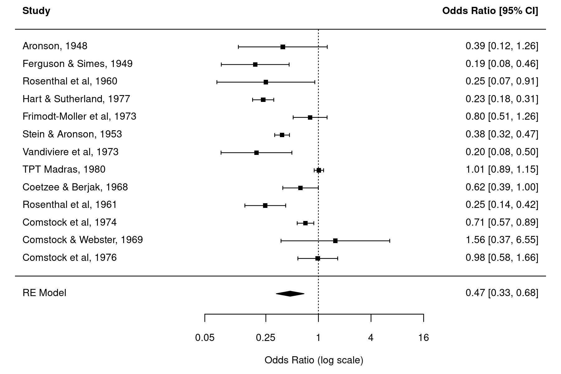
Then we can create the forest plot with:
forest(res, atransf=exp, xlim=c(-8,6),
       at=log(c(0.05, 0.25, 1, 4, 16)), psize=1)
The estimated log odds ratios of the individual studies and the pooled estimate of the random-effects model are back-transformed using exponentiation for easier interpretation (to be precise, atransf=exp does an axis transformation which results in a log scale for the x-axis and symmetric looking CIs).

The CIs of the individual studies are so-called Wald-type confidence intervals, which are computed with $y_i \pm 1.96 \sqrt{v_i}$, where $y_i$ are the observed log odds ratios and $v_i$ the corresponding sampling variances, which are then back-transformed via exponentiation. We can also obtain these CIs as follows:
summary(dat, transf=exp)[c("yi", "ci.lb", "ci.ub")]
       yi  ci.lb  ci.ub
1  0.3911 0.1212 1.2619
2  0.1890 0.0773 0.4621
3  0.2500 0.0688 0.9085
4  0.2331 0.1763 0.3082
5  0.8032 0.5138 1.2556
6  0.3836 0.3156 0.4662
7  0.1952 0.0767 0.4966
8  1.0121 0.8940 1.1458
9  0.6239 0.3908 0.9961
10 0.2463 0.1438 0.4219
11 0.7112 0.5711 0.8856
12 1.5630 0.3731 6.5476
13 0.9828 0.5816 1.6607
However, Wald-type CIs are approximate CIs that may not actually have the chosen coverage probability (i.e., they may cover the true outcomes more or less often than 95% of the times). For many outcome measures, we can compute 'exact' confidence intervals that are guaranteed to have the desired coverage probability (or a coverage probability that is at least as large as the chosen confidence level).
Using the same principle underlying Fisher's exact test (which makes use of the hypergeometric distribution), one can also compute exact CIs for the odds ratios in the individual 2x2 tables (which requires the use of the non-central hypergeometric distribution) as follows:
tmp <- lapply(split(dat, dat$trial), FUN = function(x)
              fisher.test(matrix(c(x[["tpos"]], x[["tneg"]],
                                   x[["cpos"]], x[["cneg"]]),
                          nrow=2, ncol=2, byrow=TRUE))$conf.int)
tmp <- do.call(rbind, tmp)
colnames(tmp) <- c("ci.lb", "ci.ub")
dat <- cbind(dat, tmp)
dfround(dat[c(1:3, 10:13)], digits=c(rep(0,3),rep(4,4)))
   trial               author year      yi     vi  ci.lb   ci.ub
1      1              Aronson 1948 -0.9387 0.3571 0.0887  1.3703
2      2     Ferguson & Simes 1949 -1.6662 0.2081 0.0633  0.4736
3      3      Rosenthal et al 1960 -1.3863 0.4334 0.0443  0.9666
4      4    Hart & Sutherland 1977 -1.4564 0.0203 0.1733  0.3094
5      5 Frimodt-Moller et al 1973 -0.2191 0.0520 0.4977  1.2827
6      6      Stein & Aronson 1953 -0.9581 0.0099 0.3138  0.4681
7      7     Vandiviere et al 1973 -1.6338 0.2270 0.0667  0.5523
8      8           TPT Madras 1980  0.0120 0.0040 0.8922  1.1481
9      9     Coetzee & Berjak 1968 -0.4717 0.0570 0.3768  1.0184
10    10      Rosenthal et al 1961 -1.4012 0.0754 0.1348  0.4276
11    11       Comstock et al 1974 -0.3408 0.0125 0.5680  0.8920
12    12   Comstock & Webster 1969  0.4466 0.5342 0.3037 10.0780
13    13       Comstock et al 1976 -0.0173 0.0716 0.5596  1.7207
Instead of the Wald-type CIs, we could choose to show these CIs in the forest plot. For consistency under this example, we may also want to use a model that directly models the $2 \times 2$ tables based on their exact likelihood under a non-central hypergeometric distribution. We can do this with:
res <- rma.glmm(measure="OR", ai=tpos, bi=tneg, ci=cpos, di=cneg, data=dat, model="CM.EL")
res
Random-Effects Model (k = 13; tau^2 estimator: ML)
Model Type: Conditional Model with Exact Likelihood

tau^2 (estimated amount of total heterogeneity): 0.3116 (SE = 0.1612)
tau (square root of estimated tau^2 value):      0.5582
I^2 (total heterogeneity / total variability):   91.4646%
H^2 (total variability / sampling variability):  11.7159

Tests for Heterogeneity:
Wld(df = 12) = 268.4283, p-val < .0001
LRT(df = 12) = 176.8738, p-val < .0001

Model Results:

estimate      se     zval    pval    ci.lb    ci.ub
 -0.7538  0.1801  -4.1860  <.0001  -1.1068  -0.4009  ***

---
Signif. codes:  0 '***' 0.001 '**' 0.01 '*' 0.05 '.' 0.1 ' ' 1
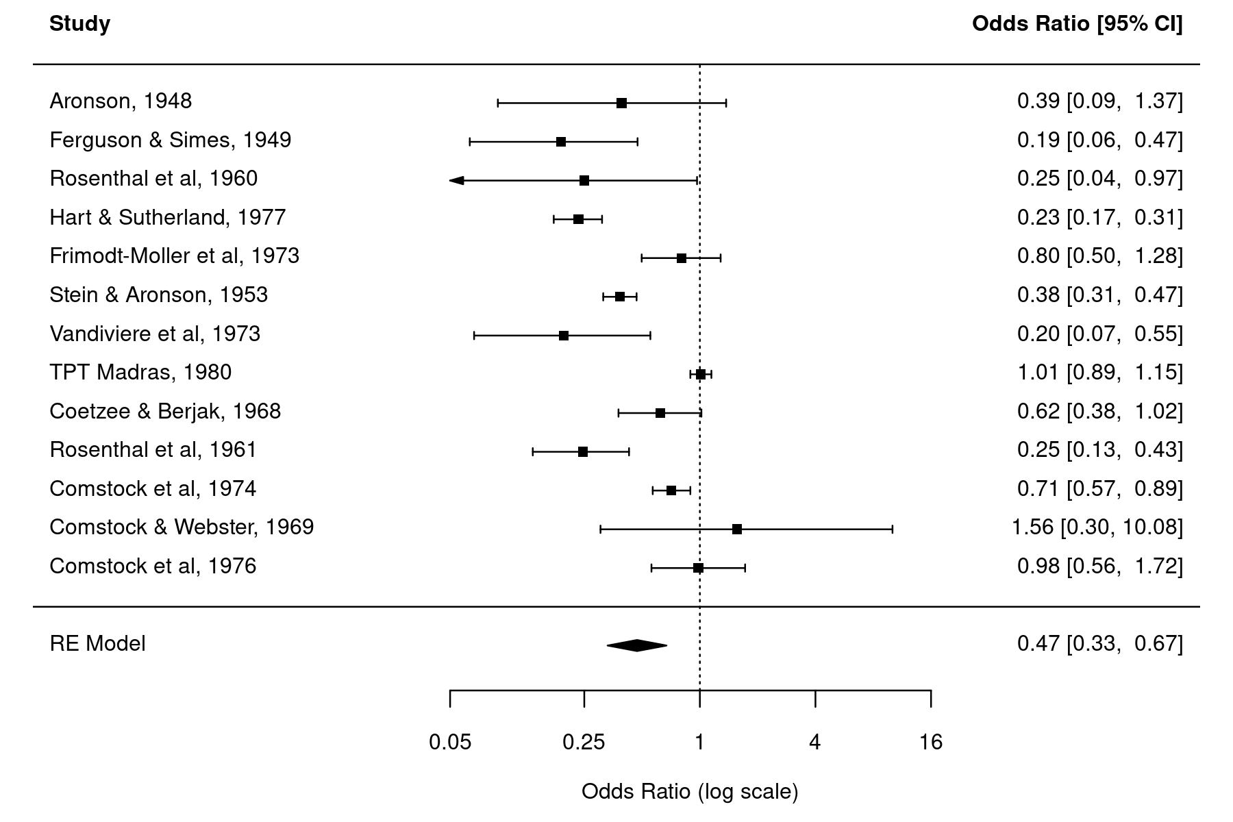
Now, we create the forest plot passing the log odds ratios and the log-transformed exact CI bounds to the forest() function and then use atransf=exp again for the axis transformation.1) A bit of space is added at the bottom where the pooled estimate based on the model above is added using addpoly().
with(dat, forest(yi, ci.lb=log(ci.lb), ci.ub=log(ci.ub), atransf=exp,
                 xlim=c(-8,6), at=log(c(0.05, 0.25, 1, 4, 16)),
                 psize=1, ylim=c(-2, res$k+3)))
abline(h=0)
addpoly(res, row=-1)

A comparison of the two forest plots shows that the latter has wider CI bounds for the individual studies, although the differences are rather negligible in most cases.2) We see somewhat more pronounced differences for smaller studies (and especially when the number of cases in the treatment and control groups are small), in which case the approximation underlying the Wald-type CI is less accurate.
The same principle as illustrated above could be used to show exact CIs for other outcome measures. However, the purpose of the forest plot is usually not to provide exact inferences about the results of the individual studies. For visualization of the individual studies and differences in their precision (as reflected in the different CI widths), using the approximate Wald-type CIs in the forest plot is often quite sufficient.