The metafor Package

After fitting a random-effects model and finding heterogeneity in the effects, meta-analysts often want to examine whether one or multiple moderator variables (i.e., predictors) are able to account for the heterogeneity (or at least part of it). Meta-regression models can be used for this purpose. A question that frequently arises in this context is how to compute an 'adjusted effect' based on such a model. This tutorial describes how to compute such adjusted effects for meta-regression models involving continuous and categorical moderators.

I will use the BCG vaccine (against tuberculosis) dataset for this tutorial. We start by computing the log risk ratios and corresponding sampling variances for the 13 trials included in this dataset.

dat <- dat.bcg
dat <- escalc(measure="RR", ai=tpos, bi=tneg, ci=cpos, di=cneg, data=dat,
              slab=paste0(author, ", ", year))
dat

   trial               author year tpos  tneg cpos  cneg ablat      alloc      yi     vi
1      1              Aronson 1948    4   119   11   128    44     random -0.8893 0.3256
2      2     Ferguson & Simes 1949    6   300   29   274    55     random -1.5854 0.1946
3      3      Rosenthal et al 1960    3   228   11   209    42     random -1.3481 0.4154
4      4    Hart & Sutherland 1977   62 13536  248 12619    52     random -1.4416 0.0200
5      5 Frimodt-Moller et al 1973   33  5036   47  5761    13  alternate -0.2175 0.0512
6      6      Stein & Aronson 1953  180  1361  372  1079    44  alternate -0.7861 0.0069
7      7     Vandiviere et al 1973    8  2537   10   619    19     random -1.6209 0.2230
8      8           TPT Madras 1980  505 87886  499 87892    13     random  0.0120 0.0040
9      9     Coetzee & Berjak 1968   29  7470   45  7232    27     random -0.4694 0.0564
10    10      Rosenthal et al 1961   17  1699   65  1600    42 systematic -1.3713 0.0730
11    11       Comstock et al 1974  186 50448  141 27197    18 systematic -0.3394 0.0124
12    12   Comstock & Webster 1969    5  2493    3  2338    33 systematic  0.4459 0.5325
13    13       Comstock et al 1976   27 16886   29 17825    33 systematic -0.0173 0.0714

The yi values are the observed log risk ratios and variable vi contains the corresponding sampling variances.

To estimate the average log risk ratio, we fit a random-effects model to these data.

res1 <- rma(yi, vi, data=dat)
res1

Random-Effects Model (k = 13; tau^2 estimator: REML)
 
tau^2 (estimated amount of total heterogeneity): 0.3132 (SE = 0.1664)
tau (square root of estimated tau^2 value):      0.5597
I^2 (total heterogeneity / total variability):   92.22%
H^2 (total variability / sampling variability):  12.86
 
Test for Heterogeneity:
Q(df = 12) = 152.2330, p-val < .0001
 
Model Results:
 
estimate      se     zval    pval    ci.lb    ci.ub
 -0.7145  0.1798  -3.9744  <.0001  -1.0669  -0.3622  ***
 
---
Signif. codes:  0 '***' 0.001 '**' 0.01 '*' 0.05 '.' 0.1 ' ' 1

To make the results easier to interpret, we can exponentiate the estimated average log risk ratio (i.e., $-0.7145$) to obtain an estimate of the average risk ratio.¹⁾ This can be done with the predict() function as follows.

predict(res1, transf=exp, digits=2)

 pred ci.lb ci.ub pi.lb pi.ub
 0.49  0.34  0.70  0.15  1.55

Hence, the estimated average risk ratio is $0.49$ (95% CI: $0.35$ to $0.70$). In other words, the data suggest that the vaccine reduces the risk of a tuberculosis infection by about 50% on average (or the risk in vaccinated groups is on average about half of the risk of non-vaccinated groups).

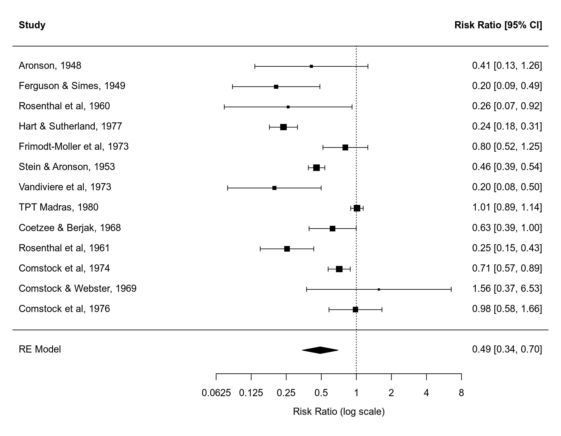
We can draw a forest plot that shows the results of the individual studies and the estimate based on the random-effects model at the bottom (the polygon shape with the center corresponding to the estimate and the ends corresponding to the confidence interval bounds).

forest(res1, xlim=c(-6.8,3.8), atransf=exp,
       at=log(c(1/16, 1/8, 1/4, 1/2, 1, 2, 4, 8)), digits=c(2L,4L))

Variable ablat in the dataset gives the absolute latitude of the study locations. The distance from the equator of the study sites may be a relevant moderator of the effectiveness of the vaccine (Bates, 1982; Colditz et al., 1994; Ginsberg, 1998). So let's fit a meta-regression model that includes this variable as a predictor.

res2 <- rma(yi, vi, mods = ~ ablat, data=dat)
res2

Mixed-Effects Model (k = 13; tau^2 estimator: REML)
 
tau^2 (estimated amount of residual heterogeneity):     0.0764 (SE = 0.0591)
tau (square root of estimated tau^2 value):             0.2763
I^2 (residual heterogeneity / unaccounted variability): 68.39%
H^2 (unaccounted variability / sampling variability):   3.16
R^2 (amount of heterogeneity accounted for):            75.62%
 
Test for Residual Heterogeneity:
QE(df = 11) = 30.7331, p-val = 0.0012
 
Test of Moderators (coefficient 2):
QM(df = 1) = 16.3571, p-val < .0001
 
Model Results:
 
         estimate      se     zval    pval    ci.lb    ci.ub
intrcpt    0.2515  0.2491   1.0095  0.3127  -0.2368   0.7397
ablat     -0.0291  0.0072  -4.0444  <.0001  -0.0432  -0.0150  ***
 
---
Signif. codes:  0 '***' 0.001 '**' 0.01 '*' 0.05 '.' 0.1 ' ' 1

The results indeed suggest that the size of the average log risk ratio is a function of the absolute latitude of the study locations.

In such a meta-regression model, there is no longer a single average effect (since the effect depends on the value of the moderator), so if we want to estimate the size of the effect, we have to specify a value for ablat. One possibility is to estimate the average risk ratio based on the average absolute latitude of the 13 trials included in the meta-analysis. We can do this as follows.²⁾

predict(res2, newmods = mean(dat$ablat), transf=exp, digits=2)

 pred ci.lb ci.ub pi.lb pi.ub
 0.49  0.39  0.60  0.27  0.87

Hence, at about 33.5 degrees absolute latitude (see mean(dat$ablat)), the estimated average risk ratio is $0.49$ (95% CI: $0.39$ to $0.60$). There is no guarantee that this predicted value will be equal to the value obtained from the random-effects model, although it often won't be too dissimilar. However, if the moderator is able to account for at least some of the heterogeneity in the effects, then the confidence interval should be narrower. We see this happening in this example (note that about 75% of the heterogeneity is accounted for by this moderator). Although one can debate the terminology, some might call this predicted effect an 'adjusted effect' based on the meta-regression model.

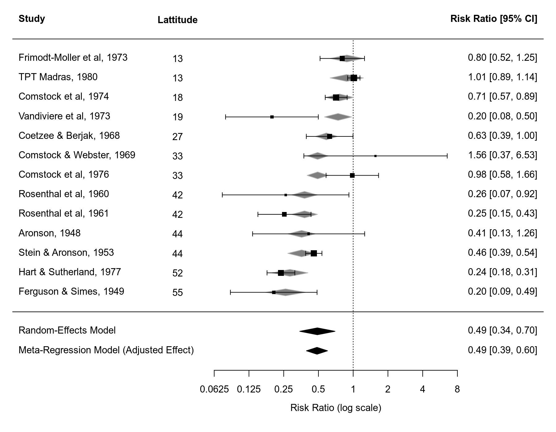
Note that if you draw a forest plot for a meta-regression model, the predicted/fitted effects corresponding to the values of the moderator of the included studies will be indicated in the plot as gray-shaded polygons.

forest(res2, xlim=c(-6.8,3.8), atransf=exp,
       at=log(c(1/16, 1/8, 1/4, 1/2, 1, 2, 4, 8)), digits=c(2L,4L),
       ilab=ablat, ilab.lab="Lattitude", ilab.xpos=-3.5,
       order=ablat, ylim=c(-3,16))
abline(h=0)
sav1 <- predict(res1)
addpoly(sav1, row=-1, mlab="Random-Effects Model")
sav2 <- predict(res2, newmods = mean(dat$ablat))
addpoly(sav2, row=-2, mlab="Meta-Regression Model (Adjusted Effect)")

In the forest plot, the values of the moderator are added as an extra column and the studies are ordered based on their absolute latitude value to make this clearer. Some extra space was also added to the forest plot to add the estimate from the standard random-effects model and the 'adjusted effect' from the meta-regression model at the bottom.

Next, let's see how this works when the moderator variable of interest is categorical. For this, we will use variable alloc, which indicates the way participants were allocated to the vaccinated versus the control group (with levels random, alternate, and systematic).

res3 <- rma(yi, vi, mods = ~ alloc, data=dat)
res3

Mixed-Effects Model (k = 13; tau^2 estimator: REML)
 
tau^2 (estimated amount of residual heterogeneity):     0.3615 (SE = 0.2111)
tau (square root of estimated tau^2 value):             0.6013
I^2 (residual heterogeneity / unaccounted variability): 88.77%
H^2 (unaccounted variability / sampling variability):   8.91
R^2 (amount of heterogeneity accounted for):            0.00%
 
Test for Residual Heterogeneity:
QE(df = 10) = 132.3676, p-val < .0001
 
Test of Moderators (coefficients 2:3):
QM(df = 2) = 1.7675, p-val = 0.4132
 
Model Results:
 
                 estimate      se     zval    pval    ci.lb   ci.ub
intrcpt           -0.5180  0.4412  -1.1740  0.2404  -1.3827  0.3468
allocrandom       -0.4478  0.5158  -0.8682  0.3853  -1.4588  0.5632
allocsystematic    0.0890  0.5600   0.1590  0.8737  -1.0086  1.1867
 
---
Signif. codes:  0 ‘***’ 0.001 ‘**’ 0.01 ‘*’ 0.05 ‘.’ 0.1 ‘ ’ 1

The intercept reflects the estimated average log risk ratio for level alternate (this is the so-called reference level), while the other two coefficients estimate how much the average log risk ratios for levels random and systematic differ from the reference level. Note that the omnibus test of these two coefficients is not actually significant ($Q_M = 1.77, \mbox{df} = 2, p = .41$), which indicates that there is insufficient evidence to conclude that the average log risk ratio differs across the three levels. However, for illustration purposes, we'll proceed with our analysis of this moderator.

First, we can compute the estimated average risk ratios for the three levels with:

predict(res3, newmods = c(0,0), transf=exp, digits=2)
predict(res3, newmods = c(1,0), transf=exp, digits=2)
predict(res3, newmods = c(0,1), transf=exp, digits=2)

  pred ci.lb ci.ub pi.lb pi.ub
1 0.60  0.25  1.41  0.14  2.57
2 0.38  0.23  0.64  0.10  1.38
3 0.65  0.33  1.28  0.17  2.53

Note: The output above was obtained with predict(res3, newmods = rbind(c(0,0), c(1,0), c(0,1)), transf=exp, digits=2), which provides the three estimates in a single line of code. However, the code above is a bit easier to read and shows how we need to set the two dummy variables (that are created for the random and systematic levels) to 0 or 1 to obtain the estimates for the three levels.

But what should we do if we want to compute an 'adjusted effect' again? In other words, what values should we plug into our model equation (and hence into newmods) to obtain such an estimate? One approach is to use the mean of the respective dummy variables. We can obtain these values from the 'model matrix' and taking means across columns (leaving out the intercept).

colMeans(model.matrix(res3))[-1]

    allocrandom allocsystematic
      0.5384615       0.3076923

Using these means for newmods then yields the 'adjusted estimate'.

predict(res3, newmods = colMeans(model.matrix(res3))[-1], transf=exp, digits=2)

 pred ci.lb ci.ub pi.lb pi.ub
 0.48  0.33  0.70  0.14  1.66

Again, this estimate is very close to the one obtained from the random-effects model. Also, since this moderator does not actually account for any heterogeneity, the confidence interval is essentially the same width as the one from the random-effects model.

What do these column means above actually represent? They are in fact proportions and indicate that 53.8% of the trials used random allocation (i.e., 7 out of the 13), 30.8% used systematic allocation (i.e., 4 out of the 13), and hence 15.4% used alternating allocation (i.e., 2 out of the 13). The predicted effect computed above is therefore an estimate for a population of studies where the relative frequencies of the different allocation methods are like those observed in the 13 trials included in the meta-analysis.

But we are not restricted to setting the proportions in this way. Another approach is to assume that the population to which we want to generalize includes studies where each allocation method is used equally often. For a three-level factor, we then need to set the values for the two dummy variables to 1/3. This yields:

predict(res3, newmods = c(1/3,1/3), transf=exp, digits=2)

 pred ci.lb ci.ub pi.lb pi.ub
 0.53  0.35  0.79  0.15  1.84

We can also consider a model that includes a mix of continuous and categorical moderators.

res4 <- rma(yi, vi, mods = ~ ablat + alloc, data=dat)
res4

Mixed-Effects Model (k = 13; tau^2 estimator: REML)
 
tau^2 (estimated amount of residual heterogeneity):     0.1446 (SE = 0.1124)
tau (square root of estimated tau^2 value):             0.3803
I^2 (residual heterogeneity / unaccounted variability): 70.11%
H^2 (unaccounted variability / sampling variability):   3.35
R^2 (amount of heterogeneity accounted for):            53.84%
 
Test for Residual Heterogeneity:
QE(df = 9) = 26.2034, p-val = 0.0019
 
Test of Moderators (coefficients 2:4):
QM(df = 3) = 11.0605, p-val = 0.0114
 
Model Results:
 
                 estimate      se     zval    pval    ci.lb    ci.ub
intrcpt            0.2932  0.4050   0.7239  0.4691  -0.5006   1.0870
ablat             -0.0273  0.0092  -2.9650  0.0030  -0.0453  -0.0092  **
allocrandom       -0.2675  0.3504  -0.7633  0.4453  -0.9543   0.4193
allocsystematic    0.0585  0.3795   0.1540  0.8776  -0.6854   0.8023
 
---
Signif. codes:  0 ‘***’ 0.001 ‘**’ 0.01 ‘*’ 0.05 ‘.’ 0.1 ‘ ’ 1

The same idea as described above can again be applied to obtain an 'adjusted effect', but now adjusted for both moderators. Again, we just need to compute column means over the model matrix and use this for newmods.

predict(res4, newmods = colMeans(model.matrix(res4))[-1], transf=exp, digits=2)

 pred ci.lb ci.ub pi.lb pi.ub
 0.47  0.36  0.62  0.22  1.05

Some may scoff at the idea of computing such an 'adjusted effect', questioning its usefulness and interpretability. I'll leave this discussion for another day. However, the method above is nothing different than what is used to compute so-called 'marginal means' (or 'least squares means', although that term is a bit outdated).

The emmeans package is a popular package that facilitates the computation of such 'estimated marginal means'. The metafor package provides a wrapper function called emmprep() that makes it possible to use the emmeans package for computing adjusted effects as shown above. As a first step, let's install and load the emmeans package:

install.packages("emmeans")
library(emmeans)

For the model that included only ablat as a predictor, we can now do the following:³⁾

sav <- emmprep(res2)
emmeans(sav, specs="1", type="response")

 1       response     SE  df asymp.LCL asymp.UCL
 overall    0.486 0.0523 Inf     0.393       0.6
 
Confidence level used: 0.95
Intervals are back-transformed from the log scale

Similarly, for the model that included the alloc factor, we can do:

sav <- emmprep(res3)
emmeans(sav, specs="1", type="response", weights="proportional")

 1       response    SE  df asymp.LCL asymp.UCL
 overall    0.481 0.092 Inf     0.331       0.7
 
Results are averaged over the levels of: alloc
Confidence level used: 0.95
Intervals are back-transformed from the log scale

Note that the default is to use equal weighting of the levels that are averaged over, so we had to explicitly set weights="proportional" to get the proportional weighting we used initially above. Therefore, for equal weighting, we can simply use:

emmeans(sav, specs="1", type="response")

 1       response    SE  df asymp.LCL asymp.UCL
 overall    0.529 0.109 Inf     0.352     0.793
 
Results are averaged over the levels of: alloc
Confidence level used: 0.95
Intervals are back-transformed from the log scale

Finally, for the model that included both ablat and alloc as predictors, we again use:

sav <- emmprep(res4)
emmeans(sav, specs="1", type="response", weights="proportional")

 1       response     SE  df asymp.LCL asymp.UCL
 overall    0.474 0.0643 Inf     0.364     0.619
 
Results are averaged over the levels of: alloc
Confidence level used: 0.95
Intervals are back-transformed from the log scale

Note that these results are identical to the ones we obtained earlier using the predict() function. However, some of the work in having to set quantitative variables to their mean value and dummy variables to their respective proportions or fractions is automatically handled when using emmprep() in combination with emmeans().

Bates, J. H. (1982). Tuberculosis: Susceptibility and resistance. American Review of Respiratory Disease, 125(3 Pt 2), 20-24.

Colditz, G. A., Brewer, T. F., Berkey, C. S., Wilson, M. E., Burdick, E., Fineberg, H. V., & Mosteller, F. (1994). Efficacy of BCG vaccine in the prevention of tuberculosis: Meta-analysis of the published literature. Journal of the American Medical Association, 271(9), 698-702.

Ginsberg, A. M. (1998). The tuberculosis epidemic: Scientific challenges and opportunities. Public Health Reports, 113(2), 128-136.