Table of Contents
Comparison of the Mantel-Haenszel Method in Different Software
The Mantel-Haenszel method is an approach for fitting meta-analytic equal-effects models when dealing with studies providing data in the form of 2x2 tables or in the form of event counts (i.e., person-time data) for two groups (Mantel & Haenszel, 1959). The method is particularly advantageous when aggregating a large number of studies with small sample sizes (the so-called sparse data or increasing strata case).
The method is available in the metafor package via the rma.mh() function. By default, the results obtained may differ slightly from those obtained via the metan function in Stata (for more details, see Harris et al., 2008; Sterne, 2009), the Review Manager (RevMan) from the Cochrane Collaboration, or Comprehensive Meta-Analysis (CMA). The reason for such discrepancies is explained further below using an illustrative dataset from a meta-analysis comparing the risk of catheter-related bloodstream infection (CRBSI) when using anti-infective-treated versus standard catheters in the acute care setting (Niel-Weise et al., 2007).
Data Preparation
The data to be used for this example are stored in the dataset dat.nielweise2007:
library(metafor)
dat <- dat.nielweise2007
dat
   study         author year ai n1i ci n2i
1      1           Bach 1996  0 116  3 117
2      2         George 1997  1  44  3  35
3      3           Maki 1997  2 208  9 195
4      4           Raad 1997  0 130  7 136
5      5          Heard 1998  5 151  6 157
6      6         Collin 1999  1  98  4 139
7      7         Hannan 1999  1 174  3 177
8      8          Marik 1999  1  74  2  39
9      9         Pierce 2000  1  97 19 103
10    10          Sheng 2000  1 113  2 122
11    11 Chatzinikolaou 2003  0  66  7  64
12    12         Corral 2003  0  70  1  58
13    13   Brun-Buisson 2004  3 188  5 175
14    14           Leon 2004  6 187 11 180
15    15          Yucel 2004  0 118  0 105
16    16        Moretti 2005  0 252  1 262
17    17           Rupp 2005  1 345  3 362
18    18           Osma 2006  4  64  1  69
Variables ai and ci indicate the number of CRBSIs in patients receiving an anti-infective or a standard catheter, respectively, while n1i and n2i indicate the total number of patients in the respective groups. Note that the number of infections was quite low in many studies, with zero cases observed in several of the treatment groups. Also, no cases (infections) were observed in either group in the Yucel (2004) study.
Mantel-Haenszel Method
An analysis of these data using the Mantel-Haenszel method can be carried out with:
res1 <- rma.mh(measure="OR", ai=ai, n1i=n1i, ci=ci, n2i=n2i, data=dat)
print(res1, digits=3)
Equal-Effects Model (k = 18)

I^2 (total heterogeneity / total variability):  5.12%
H^2 (total variability / sampling variability): 1.05

Test for Heterogeneity:
Q(df = 16) = 16.864, p-val = 0.394

Model Results (log scale):

estimate     se    zval   pval   ci.lb   ci.ub
  -1.209  0.222  -5.434  <.001  -1.645  -0.773

Model Results (OR scale):

estimate  ci.lb  ci.ub
   0.299  0.193  0.462

Cochran-Mantel-Haenszel Test:    CMH = 32.214, df = 1,  p-val < 0.001
Tarone's Test for Heterogeneity: X^2 = 25.679, df = 16, p-val = 0.059
Therefore, the odds ratio is estimated to be .299 (with 95% CI: 0.193 to 0.462). In other words, the odds of an infection are estimated to be approximately 70% lower (i.e., $(1 - .299) \times 100%$) in patients receiving an anti-infective-treated catheter instead of a standard catheter. The overall effect is clearly statistically significant (with both the Wald-type z-test and the Cochran-Mantel-Haenszel chi-square test in close agreement). The Q-test for heterogeneity is not significant ($Q(16) = 16.86, p = .39$), although Tarone's test is suggestive of potential heterogeneity.
Results from Stata
The same analysis run in Stata using the metan command (with default settings) yields the following results:
           Study     |     OR    [95% Conf. Interval]     % Weight
---------------------+---------------------------------------------------
Bach (1996)          |  0.140       0.007     2.749          3.93
Brun-Buisson (2004)  |  0.551       0.130     2.342          5.77
Chatzinikolaou (2003 |  0.058       0.003     1.031          8.56
Collin (1999)        |  0.348       0.038     3.162          3.71
Corral (2003)        |  0.272       0.011     6.801          1.84
George (1997)        |  0.248       0.025     2.497          3.70
Hannan (1999)        |  0.335       0.035     3.255          3.35
Heard (1998)         |  0.862       0.257     2.886          6.44
Leon (2004)          |  0.509       0.184     1.408         12.29
Maki (1997)          |  0.201       0.043     0.941         10.42
Marik (1999)         |  0.253       0.022     2.887          2.93
Moretti (2005)       |  0.345       0.014     8.514          1.66
Osma (2006)          |  4.533       0.493    41.683          1.02
Pierce (2000)        |  0.046       0.006     0.351         20.65
Raad (1997)          |  0.066       0.004     1.170          8.27
Rupp (2005)          |  0.348       0.036     3.360          3.31
Sheng (2000)         |  0.536       0.048     5.990          2.16
Yucel (2004)         |  (Excluded)
---------------------+---------------------------------------------------
M-H pooled OR        |  0.317       0.208     0.483        100.00
---------------------+---------------------------------------------------

  Heterogeneity chi-squared =  16.41 (d.f. = 16) p = 0.425
  I-squared (variation in OR attributable to heterogeneity) =   2.5%

  Test of OR=1 : z=   5.36 p = 0.000
The following forest plot is also generated:
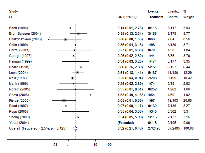
Note that the estimated overall odds ratio (and corresponding CI) is slightly different than the one obtained earlier. Also, the z-test of the overall effect and the chi-square test for heterogeneity are slightly different.
Results from RevMan
After entering the same data into the Review Manager and running the analogous analysis yields the following results:

These results match what is reported by Stata and are again slightly different compared to the results obtained with metafor.
Results from CMA
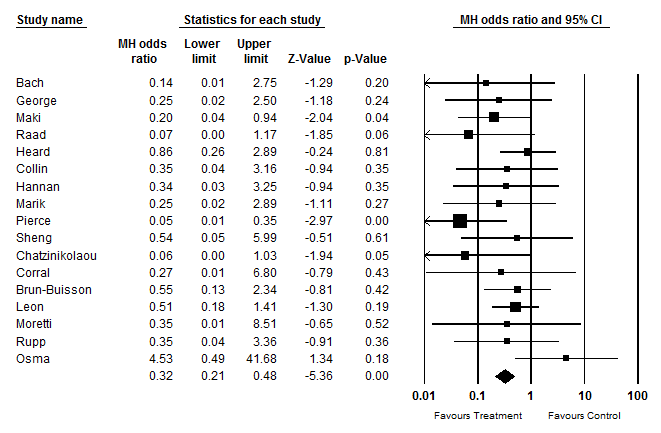
Finally, the figure below shows the results from Comprehensive Meta-Analysis (CMA). These results match those obtained with Stata and RevMan and differ slightly from those obtained with metafor.
Reason for the Difference
The results differ because studies with zero cases in either group are handled by default in a different way in metafor compared to Stata, RevMan, and CMA. To understand this better, note that the Mantel-Haenszel method itself does not require the calculation of the observed outcomes of the individual studies (in the present example, the observed (log) odds ratios of the $k$ studies) and instead directly makes use of the 2×2 table counts. Zero cells are not a problem (except in some extreme cases, such as when there are zero cases in one or both groups across all of the 2×2 tables). Therefore, it is unnecessary to add some constant to the cell counts of a study with zero cases in either group. However, both Stata, RevMan, and CMA apply an adjustment (often called a continuity correction) to the cell counts in such studies (but studies with zero cases in both groups are dropped/excluded from the method). In particular, 1/2 is added to each of the cells of the 2×2 table in such studies before applying the Mantel-Haenszel method.
By default, metafor uses this adjustment when calculating the observed outcomes (the observed log odds ratios) of the $k$ studies (here, zero cells can be problematic, so adding a constant value to the cell counts ensures that all $k$ values can be calculated). Also, similarly, studies with zero cases in both groups are automatically dropped/excluded. However, when applying the Mantel-Haenszel method, no adjustment to the cell counts is made, since this is not necessary (and in fact can increase the bias in the Mantel-Haenszel method – see Bradburn et al., 2007).
We can, however, adjust the settings, so that metafor also applies the cell count adjustment, not only when calculating the observed outcomes, but also when carrying out the computations of the Mantel-Haenszel method. For this, we have to adjust the defaults of the add, to, and drop00 arguments (see the documentation of the escalc() and rma.mh() functions for further details). In particular, we could use:
res2 <- rma.mh(measure="OR", ai=ai, n1i=n1i, ci=ci, n2i=n2i, data=dat, add=c(1/2,1/2), to=c("only0","only0"), drop00=c(TRUE,TRUE))
print(res2, digits=3)
Equal-Effects Model (k = 17)

I^2 (total heterogeneity / total variability):  2.48%
H^2 (total variability / sampling variability): 1.03

Test for Heterogeneity:
Q(df = 16) = 16.406, p-val = 0.425

Model Results (log scale):

estimate     se    zval   pval   ci.lb   ci.ub
  -1.149  0.214  -5.356  <.001  -1.569  -0.728

Model Results (OR scale):

estimate  ci.lb  ci.ub
   0.317  0.208  0.483

Cochran-Mantel-Haenszel Test:    CMH = 30.919, df = 1,  p-val < 0.001
Tarone's Test for Heterogeneity: X^2 = 22.033, df = 16, p-val = 0.142
These are the exact same results as obtained with Stata, RevMan, and CMA. However, the results of Bradburn et al. (2007) suggest that the 1/2 adjustment should only be used with caution when applying the Mantel-Haenszel method. Also, alternative correction factors could be considered, which may actually lead to more accurate results (see Sweeting et al., 2004). Finally, the findings by Bradburn et al. (2007) suggest that Peto's method (as implemented in the rma.peto() function) can actually give the least biased results and may be preferable when events are rare (as long as treatment and control groups are of approximately equal size within trials and the true odds ratio underlying the studies is not very large).
References
Bradburn, M. J., Deeks, J. J., Berlin, J. A., & Localio, A. R. (2007). Much ado about nothing: A comparison of the performance of meta-analytical methods with rare events. Statistics in Medicine, 26(1), 53–77.
Harris, R. J., Bradburn, M. J., Deeks, J. J., Harbord, R. M., Altman, D. G., & Sterne, J. A. C. (2008). metan: Fixed- and random-effects meta-analysis. The Stata Journal, 8(1), 3–28. URL: http://www.stata-journal.com/article.html?article=sbe24_2
Mantel, N., & Haenszel, W. (1959). Statistical aspects of the analysis of data from retrospective studies of disease. Journal of the National Cancer Institute, 22(4), 719–748.
Niel-Weise, B. S., Stijnen, T., & van den Broek, P. J. (2007). Anti-infective-treated central venous catheters: A systematic review of randomized controlled trials. Intensive Care Medicine, 33(12), 2058–2068.
Review Manager (RevMan) [Computer program] (Version 5.3). Copenhagen: The Nordic Cochrane Centre, The Cochrane Collaboration, 2012. URL: http://tech.cochrane.org/Revman
Sterne, J. A. C. (Ed.) (2009). Meta-analysis in Stata: An updated collection from the Stata Journal. Stata Press, College Station, TX.
Sweeting, M. J., Sutton, A. J., & Lambert, P. C. (2004). What to add to nothing? Use and avoidance of continuity corrections in meta-analysis of sparse data. Statistics in Medicine, 23(9), 1351–1375.