The metafor Package

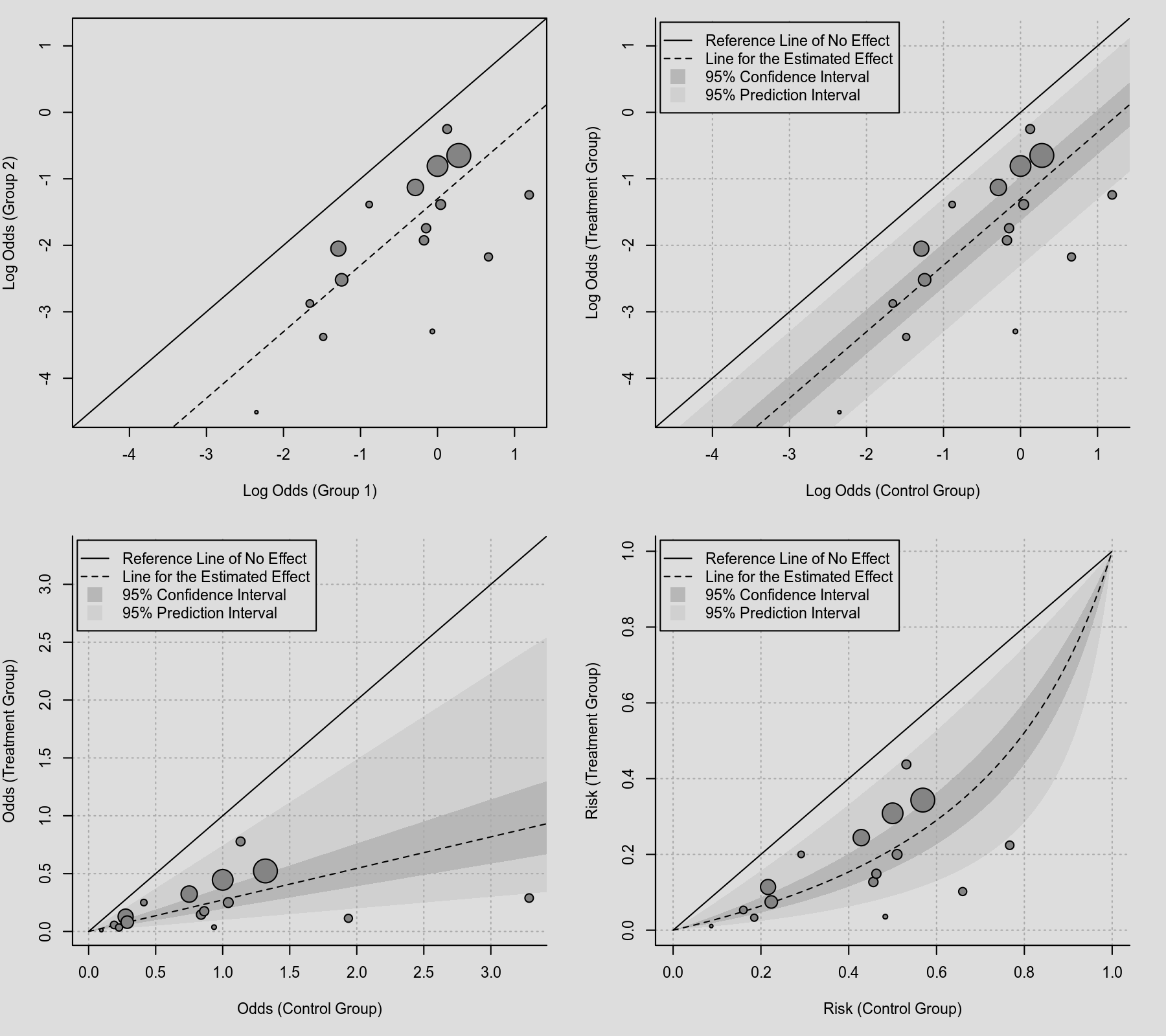
In a L'Abbé plot (based on L'Abbé, Detsky, & O'Rourke, 1987), the arm-level outcomes for two groups (e.g., treatment and control groups) are plotted against each other. The example below is based on a meta-analysis examining the effectiveness of a particular treatment (topical plus systemic antibiotics) for preventing respiratory tract infections. Since the meta-analysis is conducted with log odds ratios, the points in the first plot show by default the log odds of a respiratory tract infection in the control group (on the x-axis) versus the treatment group (on the y-axis). Points falling on the solid diagonal line represent studies where the log odds of infection did not differ between the two groups. Points falling below this line represent studies where the log odds were lower in the treated group compared to the control group. The dashed line indicates the estimated effect based on the fitted model (which is linear on the log odds scale). The size of the points is an inverse function of the precision of the estimates (so larger points correspond to more precise estimates). The next plots then illustrate some customization of such plots, including the transformation of the values on the x- and y-axes to odds and risks. Confidence and prediction interval regions are also added.

library(metafor)
 
### fit random-effects model
dat <- dat.damico2009
res <- rma(measure="OR", ai=xt, n1i=nt, ci=xc, n2i=nc, data=dat)
 
### set up 2x2 array for plotting
par(mfrow=c(2,2))
 
### decrease the overall point sizes a bit
par(cex=0.7)
 
### default plot with log odds on the x- and y-axis
labbe(res)
 
### plot with some customization
labbe(res, ci=TRUE, pi=TRUE, grid=TRUE, legend=TRUE, bty="l",
      xlab="Log Odds (Control Group)", ylab="Log Odds (Treatment Group)")
 
### plot with odds values on the x- and y-axis and some customization
labbe(res, ci=TRUE, pi=TRUE, grid=TRUE, legend=TRUE, bty="l",
      transf=exp, xlab="Odds (Control Group)", ylab="Odds (Treatment Group)")
 
### plot with risk values on the x- and y-axis and some customization
labbe(res, ci=TRUE, pi=TRUE, grid=TRUE, legend=TRUE, bty="l",
      transf=plogis, lim=c(0,1), xlab="Risk (Control Group)",
      ylab="Risk (Treatment Group)")

L'Abbé, K. A., Detsky, A. S., & O'Rourke, K. (1987). Meta-analysis in clinical research. Annals of Internal Medicine, 107(2), 224–233. https://doi.org/10.7326/0003-4819-107-2-224