The metafor Package

In some situations, we may want to model the association between the observed effect sizes / outcomes and some continuous moderator/predictor of interest in a more flexible manner than simply assuming a linear relationship. Below, I illustrate the use of polynomial and spline models for this purpose.

A data frame containing the data for this example can be created with:

dat <- structure(list(yi = c(0.99, 0.54, -0.01, 1.29, 0.66, -0.12, 1.18,
-0.23, 0.03, 0.73, 1.27, 0.38, -0.19, 0.01, 0.31, 1.41, 1.32, 1.22, 1.24,
-0.05, 1.17, -0.17, 1.29, -0.07, 0.04, 1.03, -0.16, 1.25, 0.27, 0.27, 0.07,
0.02, 0.7, 1.64, 1.66, 1.4, 0.76, 0.8, 1.91, 1.27, 0.62, -0.29, 0.17, 1.05,
-0.34, -0.21, 1.24, 0.2, 0.07, 0.21, 0.95, 1.71, -0.11, 0.17, 0.24, 0.78,
1.04, 0.2, 0.93, 1, 0.77, 0.47, 1.04, 0.22, 1.42, 1.24, 0.15, -0.53, 0.73,
0.98, 1.43, 0.35, 0.64, -0.09, 1.06, 0.36, 0.65, 1.05, 0.97, 1.28), vi =
c(0.018, 0.042, 0.031, 0.022, 0.016, 0.013, 0.066, 0.043, 0.092, 0.009,
0.018, 0.034, 0.005, 0.005, 0.015, 0.155, 0.004, 0.124, 0.048, 0.006, 0.134,
0.022, 0.004, 0.043, 0.071, 0.01, 0.006, 0.128, 0.1, 0.156, 0.058, 0.044,
0.098, 0.154, 0.117, 0.013, 0.055, 0.034, 0.152, 0.022, 0.134, 0.038, 0.119,
0.145, 0.037, 0.123, 0.124, 0.081, 0.005, 0.026, 0.018, 0.039, 0.062, 0.012,
0.132, 0.02, 0.138, 0.065, 0.005, 0.013, 0.101, 0.051, 0.011, 0.018, 0.012,
0.059, 0.111, 0.073, 0.047, 0.01, 0.007, 0.055, 0.019, 0.104, 0.056, 0.006,
0.094, 0.009, 0.008, 0.02 ), xi = c(9.4, 6.3, 1.9, 14.5, 8.4, 1.8, 11.3,
4.8, 0.7, 8.5, 15, 11.5, 4.5, 4.3, 4.3, 14.7, 11.4, 13.4, 11.5, 0.1, 12.3,
1.6, 14.6, 5.4, 2.8, 8.5, 2.9, 10.1, 0.2, 6.1, 4, 5.1, 12.4, 10.1, 13.3,
12.4, 7.6, 12.6, 12, 15.5, 4.9, 0.2, 6.4, 9.4, 1.7, 0.5, 8.4, 0.3, 4.3, 1.7,
15.2, 13.5, 6.4, 3.8, 8.2, 11.3, 11.9, 7.1, 9, 9.9, 7.8, 5.5, 9.9, 2.6,
15.5, 15.3, 0.2, 3.2, 10.1, 15, 10.3, 0, 8.8, 3.6, 15, 6.1, 3.4, 10.2, 10.1,
13.7)), class = "data.frame", row.names = c(NA, -80L))

We can inspect the first 10 rows of this dataset with:

head(dat, 10)

      yi    vi   xi
1   0.99 0.018  9.4
2   0.54 0.042  6.3
3  -0.01 0.031  1.9
4   1.29 0.022 14.5
5   0.66 0.016  8.4
6  -0.12 0.013  1.8
7   1.18 0.066 11.3
8  -0.23 0.043  4.8
9   0.03 0.092  0.7
10  0.73 0.009  8.5

Variable yi contains the observed outcomes, vi the corresponding sampling variances, and xi is the predictor of interest.

Let's examine a scatterplot of these data, with the observed outcome on the y-axis, the predictor on the x-axis, and the size of the points is drawn proportional to the inverse standard error (such that more precise estimates are reflected by larger points).

plot(dat$xi, dat$yi, pch=19, cex=.14/sqrt(dat$vi),
     xlab="Predictor", ylab="Observed Outcome", main="Scatterplot")

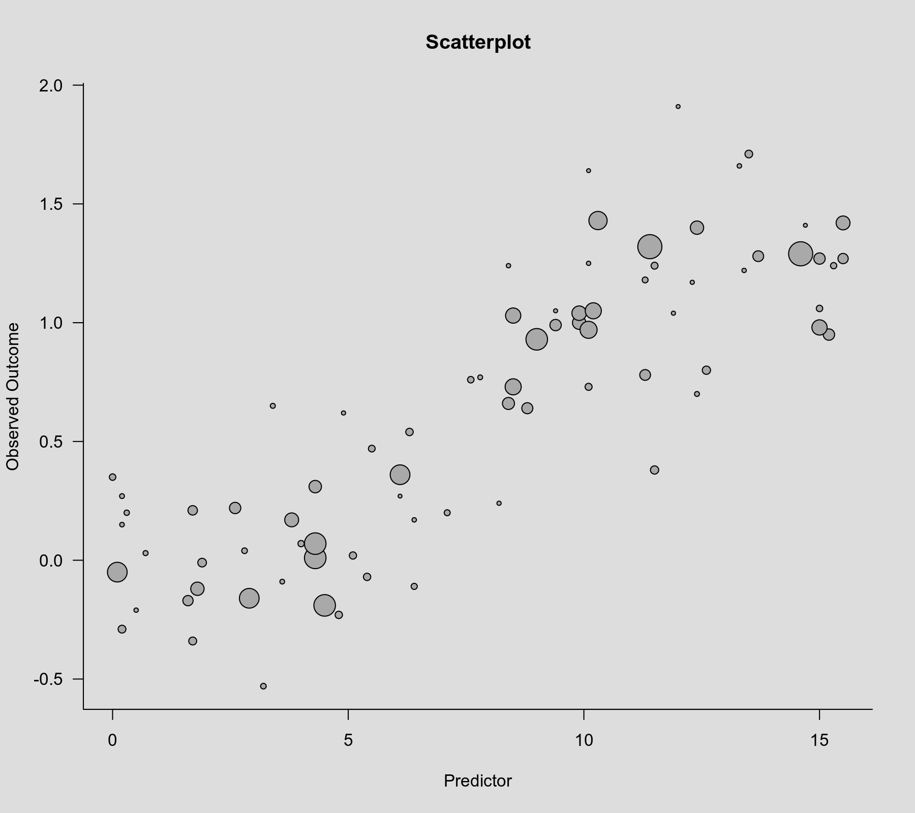
There is clearly an increasing relationship between the size of the outcomes and the values of the predictor.

We will start with fitting a linear meta-regression model to these data. After loading the metafor package, we can do this with:

library(metafor)
res.lin <- rma(yi, vi, mods = ~ xi, data=dat)
res.lin

Mixed-Effects Model (k = 80; tau^2 estimator: REML)
 
tau^2 (estimated amount of residual heterogeneity):     0.0513 (SE = 0.0133)
tau (square root of estimated tau^2 value):             0.2264
I^2 (residual heterogeneity / unaccounted variability): 72.92%
H^2 (unaccounted variability / sampling variability):   3.69
R^2 (amount of heterogeneity accounted for):            82.88%
 
Test for Residual Heterogeneity:
QE(df = 78) = 303.4429, p-val < .0001
 
Test of Moderators (coefficient 2):
QM(df = 1) = 224.2464, p-val < .0001
 
Model Results:
 
         estimate      se     zval    pval    ci.lb    ci.ub
intrcpt   -0.2126  0.0655  -3.2461  0.0012  -0.3409  -0.0842   **
xi         0.1058  0.0071  14.9749  <.0001   0.0919   0.1196  ***
 
---
Signif. codes:  0 ‘***’ 0.001 ‘**’ 0.01 ‘*’ 0.05 ‘.’ 0.1 ‘ ’ 1

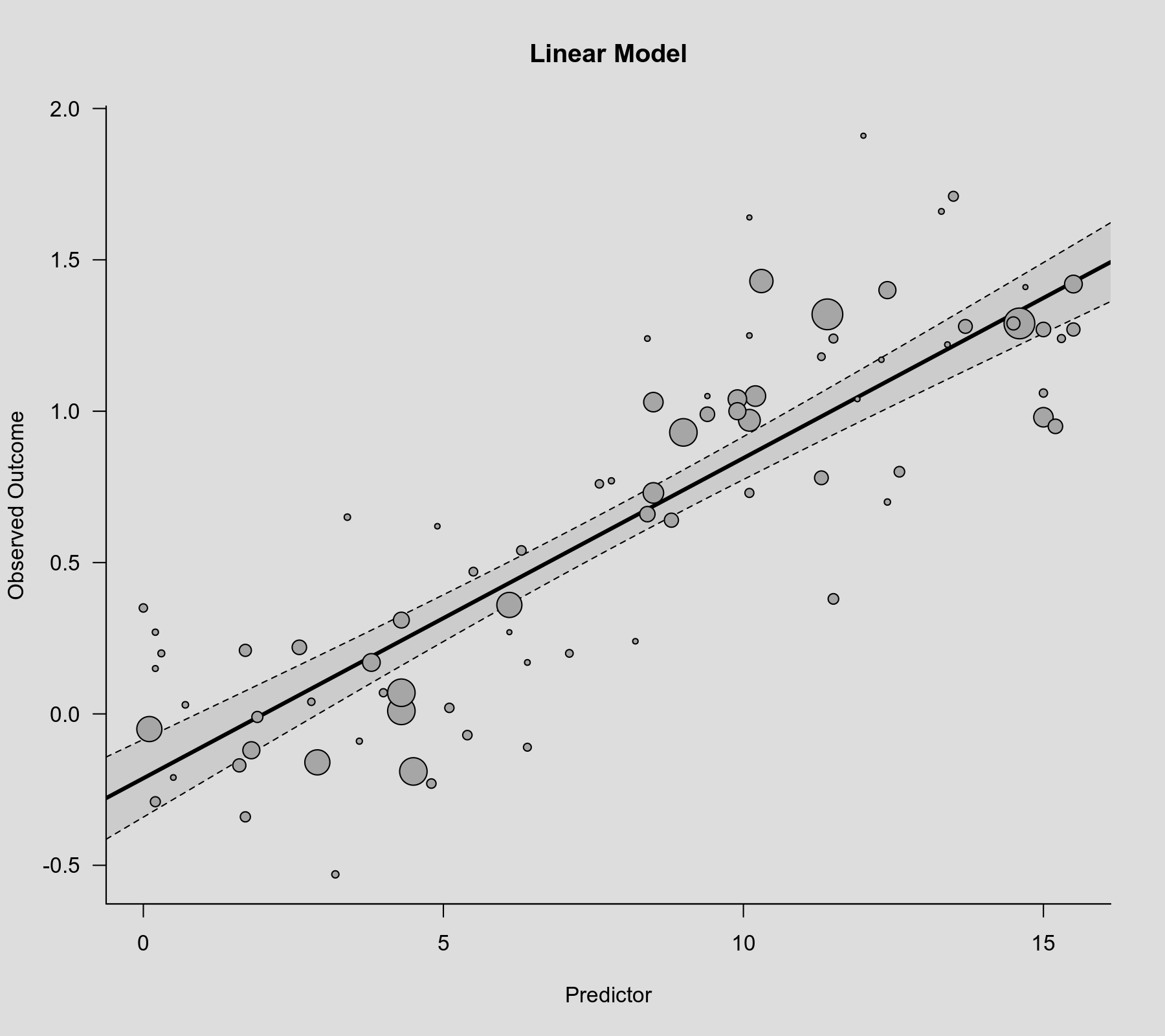
The relationship is clearly significant ($p < .0001$ for the coefficient corresponding to xi). We can visualize the linear association that is implied by this model by computing the predicted average outcome for increasing values of the predictor variable and then adding the regression line to the scatterplot. The bounds of the pointwise 95% confidence intervals for the predicted values are reflected by the gray-shaded area.

plot(dat$xi, dat$yi, pch=19, cex=.14/sqrt(dat$vi), col="gray50",
     xlab="Predictor", ylab="Observed Outcome", main="Linear Model")
xs <- seq(-1, 16, length=500)
sav <- predict(res.lin, newmods=xs)
polygon(c(xs, rev(xs)), c(sav$ci.lb, rev(sav$ci.ub)), col=rgb(0,0,0,.2), border=NA)
lines(xs, sav$pred, lwd=3)

The association between the outcome and the predictor appears to be non-linear, with the outcome barely increasing for low values of the predictor, then a steeper slope for values around the center, which then eventually seems to flatten out at the top. We could try to approximate such a relationship with a cubic polynomial model. Using the poly() function, we can easily fit such a model as follows.

res.cub <- rma(yi, vi, mods = ~ poly(xi, degree=3, raw=TRUE), data=dat)
res.cub

Mixed-Effects Model (k = 80; tau^2 estimator: REML)
 
tau^2 (estimated amount of residual heterogeneity):     0.0281 (SE = 0.0089)
tau (square root of estimated tau^2 value):             0.1677
I^2 (residual heterogeneity / unaccounted variability): 58.83%
H^2 (unaccounted variability / sampling variability):   2.43
R^2 (amount of heterogeneity accounted for):            90.60%
 
Test for Residual Heterogeneity:
QE(df = 76) = 171.5545, p-val < .0001
 
Test of Moderators (coefficients 2:4):
QM(df = 3) = 357.6414, p-val < .0001
 
Model Results:
 
                                   estimate      se     zval    pval    ci.lb    ci.ub
intrcpt                              0.0563  0.0998   0.5644  0.5725  -0.1392   0.2518
poly(xi, degree = 3, raw = TRUE)1   -0.1431  0.0551  -2.5995  0.0093  -0.2510  -0.0352   **
poly(xi, degree = 3, raw = TRUE)2    0.0417  0.0081   5.1476  <.0001   0.0258   0.0576  ***
poly(xi, degree = 3, raw = TRUE)3   -0.0018  0.0003  -5.3850  <.0001  -0.0025  -0.0011  ***
 
---
Signif. codes:  0 ‘***’ 0.001 ‘**’ 0.01 ‘*’ 0.05 ‘.’ 0.1 ‘ ’ 1

To visualize this association, we can again draw a scatterplot with the model-implied regression line.

plot(dat$xi, dat$yi, pch=19, cex=.14/sqrt(dat$vi), col="gray50",
     xlab="Predictor", ylab="Observed Outcome", main="Cubic Polynomial")
sav <- predict(res.cub, newmods=unname(poly(xs, degree=3, raw=TRUE)))
polygon(c(xs, rev(xs)), c(sav$ci.lb, rev(sav$ci.ub)), col=rgb(0,0,0,.2), border=NA)
lines(xs, sav$pred, lwd=3)

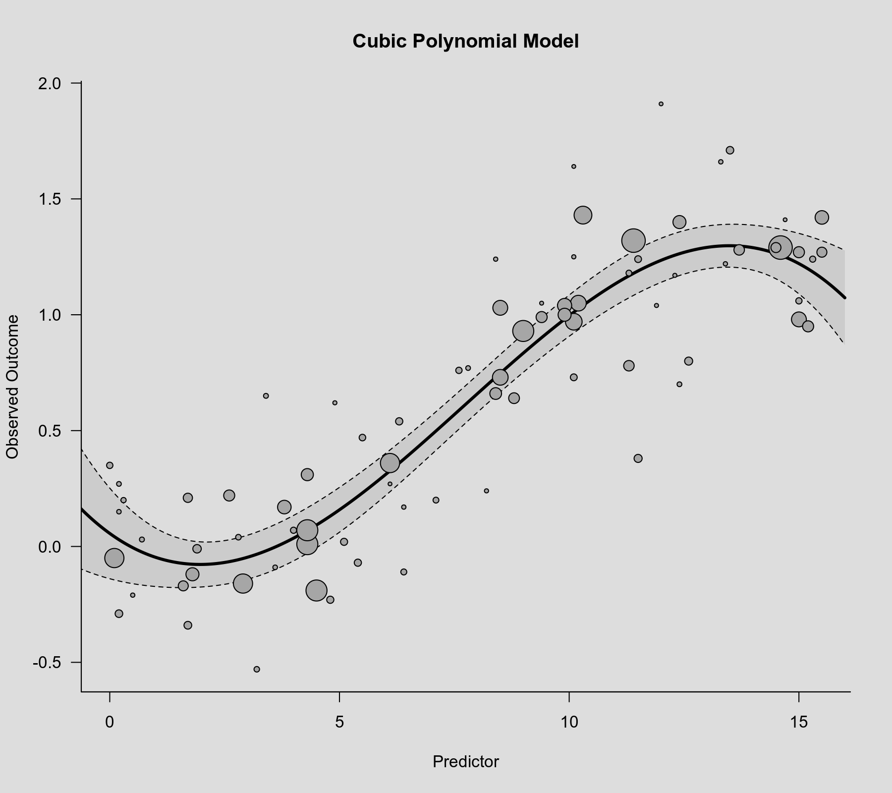
The model does appear to capture the non-linearity in the association. However, a general problem with polynomial models of this type is that they often suggest nonsensical patterns for very low or very high values of the predictor. In this case, the model suggests an initial decrease at the low end and a drop at the high end, which might not be realistic.

As an alternative approach, we could consider fitting a spline model. One popular type of model of this type consists of a series of piecewise cubic polynomials (Stone & Koo, 1985). Such a 'restricted cubic spline' model can be easily fitted with the help of the rms package. For this, we need to choose the number of 'knots', which are the positions where the piecewise cubic polynomials are connected. Here, I choose 4 knots, which yields a model with the same number of parameters are the cubic polynomial model we fitted above.

library(rms)
res.rcs <- rma(yi, vi, mods = ~ rcs(xi, 4), data=dat)
res.rcs

Mixed-Effects Model (k = 80; tau^2 estimator: REML)
 
tau^2 (estimated amount of residual heterogeneity):     0.0262 (SE = 0.0085)
tau (square root of estimated tau^2 value):             0.1619
I^2 (residual heterogeneity / unaccounted variability): 57.08%
H^2 (unaccounted variability / sampling variability):   2.33
R^2 (amount of heterogeneity accounted for):            91.24%
 
Test for Residual Heterogeneity:
QE(df = 76) = 165.4692, p-val < .0001
 
Test of Moderators (coefficients 2:4):
QM(df = 3) = 374.5340, p-val < .0001
 
Model Results:
 
                estimate      se     zval    pval    ci.lb    ci.ub
intrcpt           0.0070  0.0902   0.0773  0.9384  -0.1698   0.1838
rcs(xi, 4)xi     -0.0242  0.0315  -0.7693  0.4417  -0.0859   0.0375
rcs(xi, 4)xi'     0.4506  0.0870   5.1777  <.0001   0.2801   0.6212  ***
rcs(xi, 4)xi''   -1.4035  0.2537  -5.5326  <.0001  -1.9007  -0.9063  ***
 
---
Signif. codes:  0 ‘***’ 0.001 ‘**’ 0.01 ‘*’ 0.05 ‘.’ 0.1 ‘ ’ 1

To compute predicted values based on this model, we first need to determine the knot positions as chosen by the rcs() function.¹⁾

knots <- attr(rcs(model.matrix(res.rcs)[,2], 4), "parms")
knots

[1]  0.200  5.295 10.100 15.000

Then we can use the rcspline.eval() function with these knot positions to compute predicted values, which we can then add to the scatterplot. The know positions are also shown in the figure as dotted vertical lines.

plot(dat$xi, dat$yi, pch=19, cex=.14/sqrt(dat$vi), col="gray50",
     xlab="Predictor", ylab="Observed Outcome", main="Spline Model")
abline(v=knots, lty="dotted")
sav <- predict(res.rcs, newmods=rcspline.eval(xs, knots, inclx=TRUE))
polygon(c(xs, rev(xs)), c(sav$ci.lb, rev(sav$ci.ub)), col=rgb(0,0,0,.2), border=NA)
lines(xs, sav$pred, lwd=3)

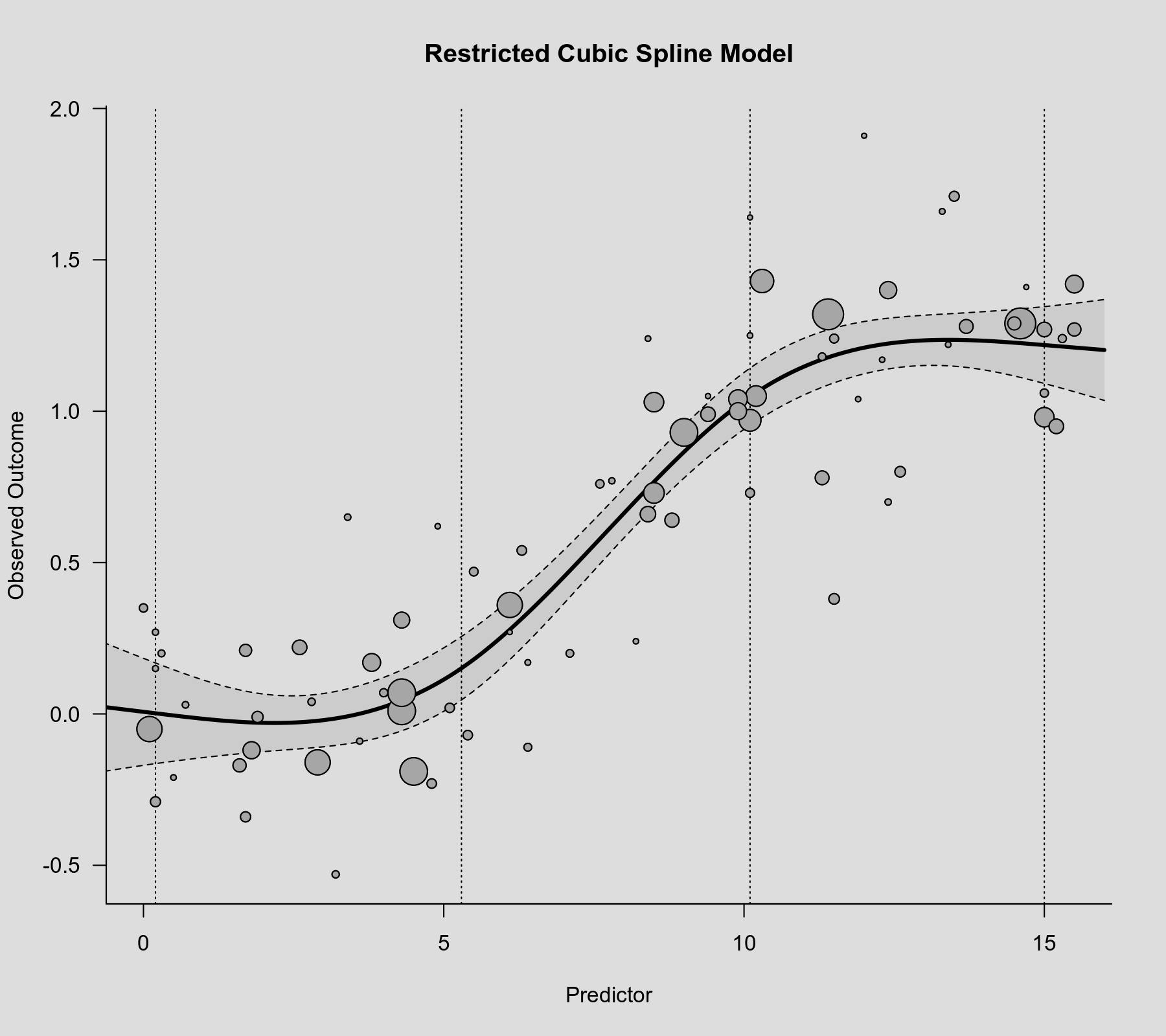
The model now suggests that the association flattens out at the lower and upper tails.

For further details on such restricted cubic spline models, see Harrell (2015). The book covers their use in the context of 'standard' regression analyses, not meta-regression, but the information provided there (e.g., on choosing the number of knots and the knot locations) is equally applicable in the present context.

Harrell, F. E., Jr. (2015). Regression modeling strategies: With applications to linear models, logistic and ordinal regression, and survival analysis (2nd ed.). New York: Springer.

Stone, C. J., & Koo, C.-K. (1985). Additive splines in statistics. In Proceedings of the Statistical Computing Section ASA. Washington, DC: American Statistical Association.