The metafor Package

The example below shows how to test and examine multiple factors and their interaction in (mixed-effects) meta-regression models.

For the example, we will use the data from the meta-analysis by Raudenbush (1984) (see also Raudenbush & Bryk, 1985) of studies examining teacher expectancy effects on pupil IQ (help(dat.raudenbush1985) provides a bit more background). The data can be loaded with:

library(metafor)
dat <- dat.raudenbush1985

I copy the dataset into dat, which is a bit shorter and therefore easier to type further below.

For illustration purposes, we will categorize the weeks variable (i.e., the number of weeks of contact prior to the expectancy induction) into three levels (0 weeks = "none", 1-9 weeks = "some", and 10+ weeks = "high"):

dat$weeks <- cut(dat$weeks, breaks=c(0,1,10,100), labels=c("none","some","high"), right=FALSE)
dat

   study               author year weeks setting tester    yi     vi
1      1     Rosenthal et al. 1974  some   group  aware  0.03 0.0156
2      2          Conn et al. 1968  high   group  aware  0.12 0.0216
3      3          Jose & Cody 1971  high   group  aware -0.14 0.0279
4      4   Pellegrini & Hicks 1972  none   group  aware  1.18 0.1391
5      5   Pellegrini & Hicks 1972  none   group  blind  0.26 0.1362
6      6    Evans & Rosenthal 1969  some   group  aware -0.06 0.0106
7      7       Fielder et al. 1971  high   group  blind -0.02 0.0106
8      8             Claiborn 1969  high   group  aware -0.32 0.0484
9      9               Kester 1969  none   group  aware  0.27 0.0269
10    10              Maxwell 1970  some   indiv  blind  0.80 0.0630
11    11               Carter 1970  none   group  blind  0.54 0.0912
12    12              Flowers 1966  none   group  blind  0.18 0.0497
13    13              Keshock 1970  some   indiv  blind -0.02 0.0835
14    14            Henrikson 1970  some   indiv  blind  0.23 0.0841
15    15                 Fine 1972  high   group  aware -0.18 0.0253
16    16              Grieger 1970  some   group  blind -0.06 0.0279
17    17 Rosenthal & Jacobson 1968  some   group  aware  0.30 0.0193
18    18   Fleming & Anttonen 1971  some   group  blind  0.07 0.0088
19    19             Ginsburg 1970  some   group  aware -0.07 0.0303

Variable yi provides the standardized mean differences and vi the corresponding sampling variances for these 19 studies. For this illustration, we will focus on variables weeks (as described above) and tester (whether the test administrator was aware or blind to the researcher-provided designations of the children's intellectual potential) as possible moderator variables.

The cut() command as used above automatically turns the weeks variable directly into a factor. Moreover, the none level is automatically set as the reference level (followed by levels some and high). To turn the tester variable into a factor and to ensure that the blind level becomes the reference level in the models to be fitted below, we can use the following command:

dat$tester <- relevel(factor(dat$tester), ref="blind")

A table with the number of factor level combinations (and margin counts) can be obtained with:

addmargins(table(dat$weeks, dat$tester))

       blind aware Sum
  none     3     2   5
  some     5     4   9
  high     1     4   5
  Sum      9    10  19

So, all factor level combinations are present in this dataset, although some of the frequencies are quite low. The results below are therefore presented for illustration purposes only.

We start by fitting a model that only contains the main effects of the two factors:

res.a1 <- rma(yi, vi, mods = ~ weeks + tester, data=dat)
res.a1

Mixed-Effects Model (k = 19; tau^2 estimator: REML)
 
tau^2 (estimated amount of residual heterogeneity):     0.0094 (SE = 0.0134)
tau (square root of estimated tau^2 value):             0.0972
I^2 (residual heterogeneity / unaccounted variability): 24.90%
H^2 (unaccounted variability / sampling variability):   1.33
R^2 (amount of heterogeneity accounted for):            49.85%
 
Test for Residual Heterogeneity:
QE(df = 15) = 24.1362, p-val = 0.0628
 
Test of Moderators (coefficients 2:4):
QM(df = 3) = 9.9698, p-val = 0.0188
 
Model Results:
 
             estimate      se     zval    pval    ci.lb    ci.ub
intrcpt        0.4020  0.1300   3.0924  0.0020   0.1472   0.6567  **
weekssome     -0.2893  0.1360  -2.1271  0.0334  -0.5558  -0.0227   *
weekshigh     -0.4422  0.1464  -3.0205  0.0025  -0.7291  -0.1552  **
testeraware   -0.0511  0.0927  -0.5512  0.5815  -0.2327   0.1305
 
---
Signif. codes:  0 '***' 0.001 '**' 0.01 '*' 0.05 '.' 0.1 ' ' 1

Let's start with the table at the bottom containing the model results. The first coefficient in the table is the model intercept ($b_0 = 0.4020$), which is the estimated average standardized mean difference for levels none and blind of the weeks and tester factors, respectively. For this combination of levels, the effect is significantly different from zero ($p = .0020$), although the 95% confidence interval ($0.1472$ to $0.6567$) indicates quite some uncertainty how large the effect really is.

The second and third coefficients correspond to the dummy variables weekssome ($b_1 = -0.2893$) and weekshigh ($b_2 = -0.4422$). These coefficients estimate how much higher/lower the average effect is for these two levels of the weeks factor compared to the reference level (i.e., none). Therefore, these coefficients directly indicate the contrast between the none and the other two levels. Both coefficients are significantly different from zero ($p = .0334$ and $p = .0025$, respectively), so the average effect is significantly different (and in fact lower) when teachers had some or a high amount of contact with the students prior to the expectancy induction (instead of no contact).

Note that we have not yet tested the weeks factor as a whole. To do so, we have to test the null hypothesis that both coefficients are equal to zero simultaneously (see also the illustration of how to test factors and linear combinations of parameters in meta-regression models). We can do this with:

anova(res.a1, btt=2:3)

Test of Moderators (coefficients 2:3):
QM(df = 2) = 9.1550, p-val = 0.0103

This is a Wald-type chi-square test with 2 degrees of freedom, indicating that the factor as a whole is in fact significant ($p = .0103$).

We have also not yet tested whether there is a difference between levels some and high of this factor. One could change the reference level of the weeks factor and refit the model to obtain this test. Alternatively, and more elegantly, we can just test the difference between these two coefficients directly. We can do this with:

anova(res.a1, X=c(0,1,-1,0))

Hypothesis:
1: weekssome - weekshigh = 0
 
Results:
   estimate     se   zval   pval
1:   0.1529 0.1016 1.5050 0.1323
 
Test of Hypothesis:
QM(df = 1) = 2.2650, p-val = 0.1323

So, we actually do not have sufficient evidence to conclude that there is a significant difference between these two levels ($p = .1323$).

We could also obtain all three pairwise comparisons simultaneously with:

anova(res.a1, X=rbind(c(0,1,0,0), c(0,0,1,0), c(0,1,-1,0)))

Hypotheses:
1:             weekssome = 0
2:             weekshigh = 0
3: weekssome - weekshigh = 0
 
Results:
   estimate     se    zval   pval
1:  -0.2893 0.1360 -2.1271 0.0334  *
2:  -0.4422 0.1464 -3.0205 0.0025 **
3:   0.1529 0.1016  1.5050 0.1323

By default, the p-values are not adjusted for multiple testing, but various adjustments are available via the adjust argument (see help(anova.rma)).

Finally, the last coefficient in the model table corresponds to the dummy variable testeraware ($b_3 = -0.0511$) and estimates how much higher/lower the average effect is for studies where the test administrator was aware of the children's designation compared to studies where the test administrator was blind. So, again, this is a contrast between these two levels. The coefficient is not significantly different from zero ($p = .5815$), so this factor does not appear to account for heterogeneity in the effects.

The output includes some additional results. First of all, the results given under Test of Moderators (coefficient(s) 2:4) is the omnibus test of coefficients 2, 3, and 4 (the first being the intercept, which is not included in the test by default). This Wald-type chi-square test is significant ($Q_M = 9.97, df = 3, p = .02$), so we can reject the null hypothesis that all of these coefficients are equal to zero (which would imply that there is no relationship between the size of the effect and these two factors). Moreover, the pseudo-$R^2$ value given suggests that roughly 50% of the total amount of heterogeneity is accounted for when including these two factors in the model. Finally, the Test for Residual Heterogeneity just falls short of being significant ($Q_E = 24.14, df = 15, p = .06$), which would suggest that there is no significant amount of residual heterogeneity in the true effects when including these two factors in the model.

Based on the fitted model, we can also obtain the estimated average effect for each combination of the factor levels. For this, we can use the predict() function, specifying how the dummy variables should be filled in. For levels none, some, and high of the weeks factor and level blind of the tester factor, we would use:

predict(res.a1, newmods=rbind(c(0,0,0),c(1,0,0),c(0,1,0)))

     pred     se   ci.lb  ci.ub   pi.lb  pi.ub
1  0.4020 0.1300  0.1472 0.6567  0.0839 0.7200
2  0.1127 0.0804 -0.0448 0.2702 -0.1345 0.3599
3 -0.0402 0.1020 -0.2401 0.1597 -0.3163 0.2359

For the same levels of the weeks factor and level aware of the tester factor, we would use:

predict(res.a1, newmods=rbind(c(0,0,1),c(1,0,1),c(0,1,1)))

     pred     se   ci.lb  ci.ub   pi.lb  pi.ub
1  0.3509 0.1297  0.0966 0.6051  0.0332 0.6685
2  0.0616 0.0735 -0.0824 0.2056 -0.1772 0.3004
3 -0.0913 0.0857 -0.2592 0.0767 -0.3452 0.1627

Note that, by default, the intercept is automatically included in the calculation of these predicted values, since the model also includes an intercept term (so only a matrix with 3 columns is specified via the newmods argument). One could also obtain the same results with:

predict(res.a1, newmods=rbind(c(1,0,0,0),c(1,1,0,0),c(1,0,1,0)))
predict(res.a1, newmods=rbind(c(1,0,0,1),c(1,1,0,1),c(1,0,1,1)))

The values under ci.lb and ci.ub are the bounds of the 95% confidence intervals, while the values under pi.lb and pi.ub are the bounds of the 95% prediction intervals (see help(predict.rma) for more details).

We can use an alternative model specification, where we leave out the model intercept:

res.a2 <- rma(yi, vi, mods = ~ 0 + weeks + tester, data=dat)
res.a2

Mixed-Effects Model (k = 19; tau^2 estimator: REML)
 
tau^2 (estimated amount of residual heterogeneity):     0.0094 (SE = 0.0134)
tau (square root of estimated tau^2 value):             0.0972
I^2 (residual heterogeneity / unaccounted variability): 24.90%
H^2 (unaccounted variability / sampling variability):   1.33
 
Test for Residual Heterogeneity:
QE(df = 15) = 24.1362, p-val = 0.0628
 
Test of Moderators (coefficients 1:4):
QM(df = 4) = 12.6719, p-val = 0.0130
 
Model Results:
 
             estimate      se     zval    pval    ci.lb   ci.ub
weeksnone      0.4020  0.1300   3.0924  0.0020   0.1472  0.6567  **
weekssome      0.1127  0.0804   1.4021  0.1609  -0.0448  0.2702
weekshigh     -0.0402  0.1020  -0.3941  0.6935  -0.2401  0.1597
testeraware   -0.0511  0.0927  -0.5512  0.5815  -0.2327  0.1305
 
---
Signif. codes:  0 '***' 0.001 '**' 0.01 '*' 0.05 '.' 0.1 ' ' 1

Note that the first three coefficients now directly correspond to the estimated average effects for levels none, some, and high of the weeks factor and level blind of the tester factor. The last (4th) coefficient again indicates how much higher/lower the average effect is when the level of the tester factor is changed to aware. Also, note that the omnibus test now includes all four coefficients by default and has a different interpretation: It is essentially testing the null hypothesis that the true average effect is zero across all factor level combinations.

The model including only the main effects of the two factors assumes that the influence of the two factors is additive. We can illustrate the implications graphically by plotting the estimated average effects for all factor level combinations:

plot(coef(res.a2)[1:3], type="o", pch=19, xlim=c(0.8,3.2), ylim=c(-0.1,0.5),
     xlab="Amount of Contact Prior to Expectancy Induction",
     ylab="Standardized Mean Difference", xaxt="n", bty="l", las=1)
axis(side=1, at=1:3, labels=c("none","some","high"))
lines(coef(res.a2)[1:3] + coef(res.a2)[4], type="o", pch=15, lty="dotted")
legend("topright", legend=c("Test Administrator Blind", "Test Administrator Aware"),
       lty=c("solid", "dotted"), pch=c(19,15), inset=0.01)
title("Estimated Average Effects based on the Additive Model")

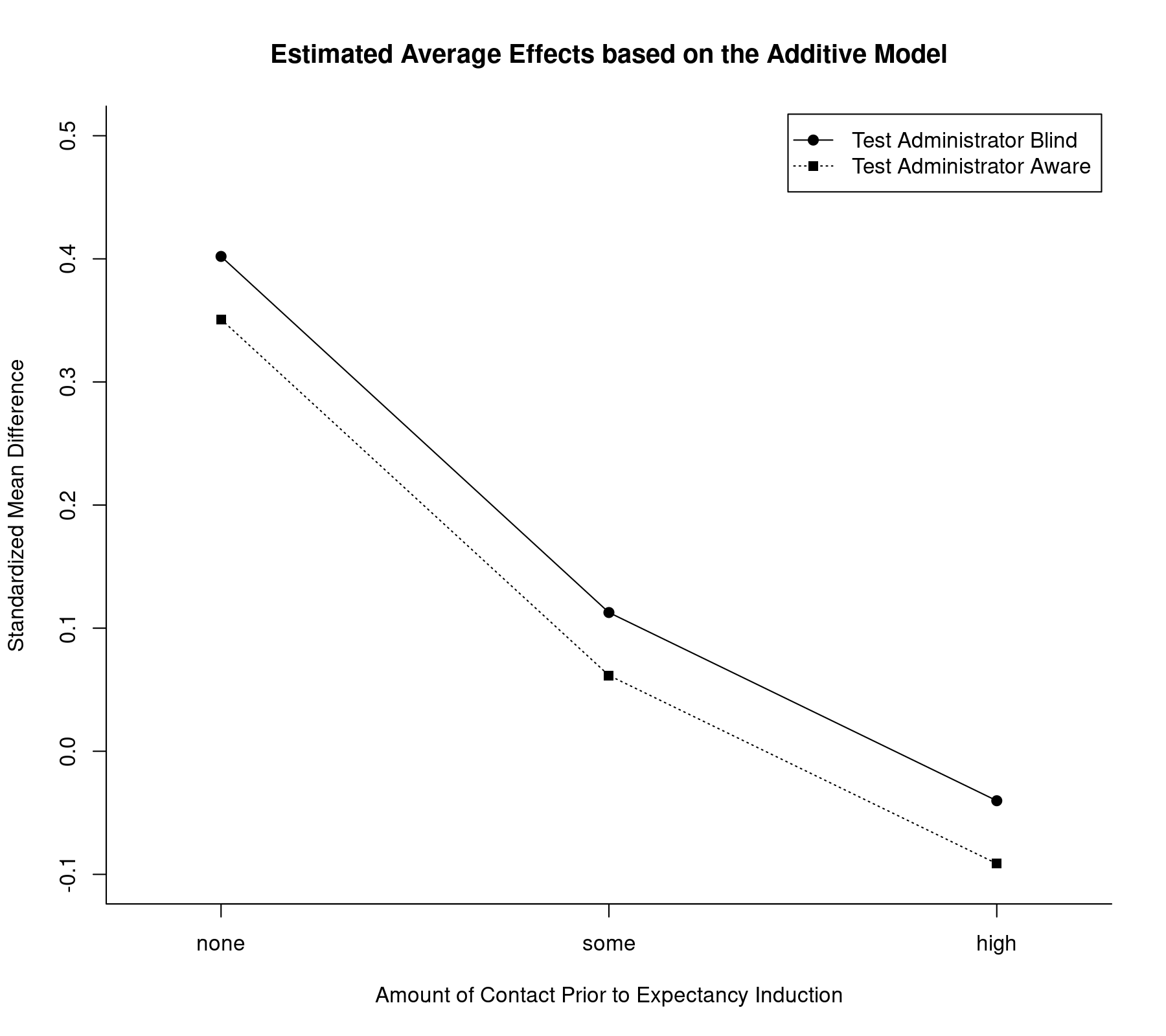
Note how the lines are parallel to each other, as expected under this model. Also, the tester factor appears to have only a minor influence on the effect as compared to the weeks factor. Finally, while we have treated weeks as a factor, the decrease in the estimated average effect appears roughly linear as we move from the none to the some and high levels. Therefore, one could also consider fitting a model where this variable is treated as a quantitative moderator. An example along those lines can be found in the discussion on how to test factors and linear combinations of parameters in mixed-effects meta-regression models.

Now let's move on to a model where we allow the two factors in the model to interact (note that it is questionable whether such a complex model should even be considered for these data; again, these analyses are used for illustration purposes only). Such a model can be fitted with:

res.i1 <- rma(yi, vi, mods = ~ weeks * tester, data=dat)
res.i1

Mixed-Effects Model (k = 19; tau^2 estimator: REML)
 
tau^2 (estimated amount of residual heterogeneity):     0.0223 (SE = 0.0214)
tau (square root of estimated tau^2 value):             0.1494
I^2 (residual heterogeneity / unaccounted variability): 42.22%
H^2 (unaccounted variability / sampling variability):   1.73
R^2 (amount of heterogeneity accounted for):            0.00%
 
Test for Residual Heterogeneity:
QE(df = 13) = 23.4646, p-val = 0.0364
 
Test of Moderators (coefficients 2:6):
QM(df = 5) = 9.3154, p-val = 0.0971
 
Model Results:
 
                       estimate      se     zval    pval    ci.lb   ci.ub
intrcpt                  0.3067  0.1857   1.6518  0.0986  -0.0572  0.6707  .
weekssome               -0.1566  0.2159  -0.7255  0.4682  -0.5797  0.2665
weekshigh               -0.3267  0.2597  -1.2584  0.2082  -0.8357  0.1822
testeraware              0.1759  0.2687   0.6547  0.5127  -0.3508  0.7026
weekssome:testeraware   -0.2775  0.3072  -0.9034  0.3663  -0.8795  0.3245
weekshigh:testeraware   -0.2634  0.3435  -0.7667  0.4433  -0.9366  0.4099
 
---
Signif. codes:  0 '***' 0.001 '**' 0.01 '*' 0.05 '.' 0.1 ' ' 1

As before, the first coefficient in the table is the model intercept ($b_0 = 0.3067$), which is the estimated average effect for levels none and blind of the weeks and tester factors, respectively. The second and third coefficients ($b_1 = -0.1566$ and $b_2 = -0.3267$, respectively) indicate how much higher/lower the estimated average effect is for levels some and high of the weeks factor when the level of the tester factor is held at blind. The fourth coefficient ($b_3 = 0.1759$) provides an estimate of how much higher/lower the average effect is for the aware level of the tester factor when the level of the weeks factor is held at none. Finally, the last two coefficients ($b_4 = -0.2775$ and $b_5 = -0.2634$, respectively) indicate how much higher/lower the contrast between the aware and blind levels of the tester factor are for levels some and high of the weeks factor (or equivalently, how much higher/lower the contrasts between the some and the none levels and the high and the none levels of the weeks factor are for level aware of the tester factor).

These last two coefficients allow the influence of the aware factor to differ across the various levels of the weeks factor (and vice-versa). Therefore, if these two coefficients are in reality both equal to zero, then there is in fact no interaction. So, in order to test whether an interaction is actually present, we just need to test these two coefficients, which we can do with:

anova(res.i1, btt=5:6)

Test of Moderators (coefficient(s) 5,6):
QM(df = 2) = 0.8576, p-val = 0.6513

Based on this Wald-type chi-square test, we find no significant evidence that an interaction is actually present ($Q_M = 0.86, df = 2, p = .65$).

Alternatively, we could use a likelihood ratio test (LRT) to test the interaction. For this, we must fit both models with maximum likelihood (ML) estimation and then conduct a model comparison:

res.a1.ml <- rma(yi, vi, mods = ~ weeks + tester, data=dat, method="ML")
res.i1.ml <- rma(yi, vi, mods = ~ weeks * tester, data=dat, method="ML")
anova(res.a1.ml, res.i1.ml)

        df    AIC     BIC    AICc logLik    LRT   pval      QE  tau^2      R^2
Full     7 8.5528 15.1639 18.7346 2.7236               23.4646 0.0000
Reduced  5 5.2247  9.9469  9.8401 2.3876 0.6719 0.7147 24.1362 0.0000 71.6487%

The results from the LRT ($\chi^2 = 0.67, df = 2, p = .71$) lead to the same conclusion.

For illustration purposes, let us however proceed with a further examination of this model. As before, the anova() function can be used to test factor levels against each other and to obtain pairwise comparisons. Also, the predict() function can be used to obtain the estimated average effect for particular factor level combinations. For example, to obtain the estimated average effect for level high of the weeks factor and level aware of the tester factor, we would use:

predict(res.i1, newmods=c(0,1,1,0,1))

     pred     se   ci.lb  ci.ub   pi.lb  pi.ub
1 -0.1074 0.1134 -0.3296 0.1148 -0.4751 0.2602

We can also make use of an alternative parameterization of the model, which is particularly useful in this context:

res.i2 <- rma(yi, vi, mods = ~ 0 + weeks:tester, data=dat)
res.i2

Mixed-Effects Model (k = 19; tau^2 estimator: REML)
 
tau^2 (estimated amount of residual heterogeneity):     0.0223 (SE = 0.0214)
tau (square root of estimated tau^2 value):             0.1494
I^2 (residual heterogeneity / unaccounted variability): 42.22%
H^2 (unaccounted variability / sampling variability):   1.73
 
Test for Residual Heterogeneity:
QE(df = 13) = 23.4646, p-val = 0.0364
 
Test of Moderators (coefficients 1:6):
QM(df = 6) = 11.9111, p-val = 0.0640
 
Model Results:
 
                       estimate      se     zval    pval    ci.lb   ci.ub
weeksnone:testerblind    0.3067  0.1857   1.6518  0.0986  -0.0572  0.6707  .
weekssome:testerblind    0.1502  0.1100   1.3646  0.1724  -0.0655  0.3658
weekshigh:testerblind   -0.0200  0.1815  -0.1102  0.9122  -0.3757  0.3357
weeksnone:testeraware    0.4827  0.1942   2.4850  0.0130   0.1020  0.8634  *
weekssome:testeraware    0.0486  0.1001   0.4851  0.6276  -0.1477  0.2448
weekshigh:testeraware   -0.1074  0.1134  -0.9476  0.3433  -0.3296  0.1148
 
---
Signif. codes:  0 '***' 0.001 '**' 0.01 '*' 0.05 '.' 0.1 ' ' 1

The table with the model results now directly provides the estimated average effect for each factor level combination. This also makes it quite easy to test particular factor level combinations against each other. For example, to test the difference between levels some and high of the weeks factor within the blind level of the tester factor, we could use:

anova(res.i2, X=c(0,1,-1,0,0,0))

Hypothesis:
1: weekssome:testerblind - weekshigh:testerblind = 0
 
Results:
   estimate     se   zval   pval
1:   0.1702 0.2122 0.8017 0.4227
 
Test of Hypothesis:
QM(df = 1) = 0.6428, p-val = 0.4227

To test the same contrast within the aware level of the tester factor, we would use:

anova(res.i2, X=c(0,0,0,0,1,-1))

Hypothesis:
1: weekssome:testeraware - weekshigh:testeraware = 0
 
Results:
   estimate     se   zval   pval
1:   0.1560 0.1513 1.0314 0.3024
 
Test of Hypothesis:
QM(df = 1) = 1.0638, p-val = 0.3024

If one were inclined to do so, one could even test all 6 factor level combinations against each other (i.e., all possible pairwise comparisons). The pairmat() function makes this relatively easy:¹⁾

anova(res.i2, X=pairmat(btt=1:6))

Hypotheses:
1:  -weeksnone:testerblind + weekssome:testerblind = 0
2:  -weeksnone:testerblind + weekshigh:testerblind = 0
3:  -weeksnone:testerblind + weeksnone:testeraware = 0
4:  -weeksnone:testerblind + weekssome:testeraware = 0
5:  -weeksnone:testerblind + weekshigh:testeraware = 0
6:  -weekssome:testerblind + weekshigh:testerblind = 0
7:  -weekssome:testerblind + weeksnone:testeraware = 0
8:  -weekssome:testerblind + weekssome:testeraware = 0
9:  -weekssome:testerblind + weekshigh:testeraware = 0
10: -weekshigh:testerblind + weeksnone:testeraware = 0
11: -weekshigh:testerblind + weekssome:testeraware = 0
12: -weekshigh:testerblind + weekshigh:testeraware = 0
13: -weeksnone:testeraware + weekssome:testeraware = 0
14: -weeksnone:testeraware + weekshigh:testeraware = 0
15: -weekssome:testeraware + weekshigh:testeraware = 0
 
Results:
    estimate     se    zval   pval
1:   -0.1566 0.2159 -0.7255 0.4682
2:   -0.3267 0.2597 -1.2584 0.2082
3:    0.1759 0.2687  0.6547 0.5127
4:   -0.2582 0.2110 -1.2237 0.2211
5:   -0.4142 0.2176 -1.9037 0.0570  .
6:   -0.1702 0.2122 -0.8017 0.4227
7:    0.3325 0.2232  1.4895 0.1364
8:   -0.1016 0.1488 -0.6828 0.4947
9:   -0.2576 0.1580 -1.6304 0.1030
10:   0.5027 0.2658  1.8910 0.0586  .
11:   0.0686 0.2073  0.3308 0.7408
12:  -0.0874 0.2140 -0.4086 0.6828
13:  -0.4341 0.2185 -1.9865 0.0470  *
14:  -0.5901 0.2249 -2.6238 0.0087 **
15:  -0.1560 0.1513 -1.0314 0.3024

As before, no adjustment to the p-values has been used for these tests, but this would probably be advisable when conducting so many tests.

We can also illustrate the results from the interaction model by plotting the estimated average effects for all factor level combinations:

plot(coef(res.i2)[1:3], type="o", pch=19, xlim=c(0.8,3.2), ylim=c(-0.1,0.5),
     xlab="Amount of Contact Prior to Expectancy Induction",
     ylab="Standardized Mean Difference", xaxt="n", bty="l", las=1)
axis(side=1, at=1:3, labels=c("none","some","high"))
lines(coef(res.i2)[4:6], type="o", pch=15, lty="dotted")
legend("topright", legend=c("Test Administrator Blind", "Test Administrator Aware"),
       lty=c("solid", "dotted"), pch=c(19,15), inset=0.01)
title("Estimated Average Effects based on the Interaction Model")

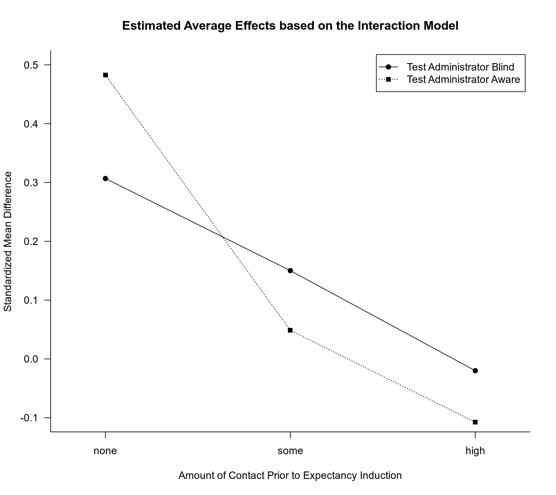
Now, the lines are no longer constrained to be parallel and in fact cross each other (but as we saw before, there is hardly any evidence to suggest that there is a significant interaction).

Raudenbush, S. W. (1984). Magnitude of teacher expectancy effects on pupil IQ as a function of the credibility of expectancy induction: A synthesis of findings from 18 experiments. Journal of Educational Psychology, 76(1), 85–97.

Raudenbush, S. W., & Bryk, A. S. (1985). Empirical Bayes meta-analysis. Journal of Educational Statistics, 10(2), 75–98.