varweighting="Johnson" so equation 6.12 from Burnham and Anderson (2002) is used for computing the standard errors (instead of 4.9), which Anderson (2008) recommends.tips:model_selection_with_glmulti_and_mumin
Table of Contents
Model Selection using the glmulti and MuMIn Packages
Information-theoretic approaches provide methods for model selection and (multi)model inference that differ quite a bit from more traditional methods based on null hypothesis testing (e.g., Anderson, 2008; Burnham & Anderson, 2002). These methods can also be used in the meta-analytic context when model fitting is based on likelihood methods. Below, I illustrate how to use the metafor package in combination with the glmulti and MuMIn packages that provide the necessary functionality for model selection and multimodel inference using an information-theoretic approach.
Data Preparation
For the example, I will use data from the meta-analysis by Bangert-Drowns et al. (2004) on the effectiveness of school-based writing-to-learn interventions on academic achievement (help(dat.bangertdrowns2004) provides a bit more background on this dataset). The data can be loaded with:
library(metafor)
dat <- dat.bangertdrowns2004
(I copy the dataset into dat, which is a bit shorter and therefore easier to type further below). We can look at the first 10 and the last 10 rows of the dataset with:
rbind(head(dat, 10), tail(dat, 10))
   id          author year grade length minutes wic feedback info pers imag meta                subject  ni    yi    vi
1   1        Ashworth 1992     4     15      NA   1        1    1    1    0    1                Nursing  60  0.65 0.070
2   2           Ayers 1993     2     10      NA   1       NA    1    1    1    0          Earth Science  34 -0.75 0.126
3   3          Baisch 1990     2      2      NA   1        0    1    1    0    1                   Math  95 -0.21 0.042
4   4           Baker 1994     4      9      10   1        1    1    0    0    0                Algebra 209 -0.04 0.019
5   5          Bauman 1992     1     14      10   1        1    1    1    0    1                   Math 182  0.23 0.022
6   6          Becker 1996     4      1      20   1        0    0    1    0    0             Literature 462  0.03 0.009
7   7     Bell & Bell 1985     3      4      NA   1        1    1    1    0    1                   Math  38  0.26 0.106
8   8         Brodney 1994     1     15      NA   1        1    1    1    0    1                   Math 542  0.06 0.007
9   9          Burton 1986     4      4      NA   0        1    1    0    0    0                   Math  99  0.06 0.040
10 10       Davis, BH 1990     1      9      10   1        0    1    1    0    0         Social Studies  77  0.12 0.052
39 39 Ross & Faucette 1994     4     15      NA   0        1    1    0    0    0                Algebra  16  0.70 0.265
40 40           Sharp 1987     4      2      15   1        0    0    1    0    1                Biology 105  0.49 0.039
41 41         Shepard 1992     2      4      NA   0        1    1    0    0    0                   Math 195  0.20 0.021
42 42         Stewart 1992     3     24       5   1        1    1    1    0    1                Algebra  62  0.58 0.067
43 43         Ullrich 1926     4     11      NA   0        1    1    0    0    0 Educational Psychology 289  0.15 0.014
44 44 Weiss & Walters 1980     4     15       3   1        0    1    0    0    0             Statistics  25  0.63 0.168
45 45           Wells 1986     1      8      15   1        0    1    1    0    1                   Math 250  0.04 0.016
46 46          Willey 1988     3     15      NA  NA        0    1    1    0    1                Biology  51  1.46 0.099
47 47          Willey 1988     2     15      NA  NA        0    1    1    0    1         Social Studies  46  0.04 0.087
48 48       Youngberg 1989     4     15      10   1        1    1    0    0    0                Algebra  56  0.25 0.072
Variable yi contains the effect size estimates (standardized mean differences) and vi the corresponding sampling variances. There are 48 rows of data in this dataset.
For illustration purposes, the following variables will be examined as potential moderators of the treatment effect (i.e., the size of the treatment effect may vary in a systematic way as a function of one or more of these variables):
- length: treatment length (in weeks)
- wic: writing tasks were completed in class (0 = no; 1 = yes)
- feedback: feedback on writing was provided (0 = no; 1 = yes)
- info: writing contained informational components (0 = no; 1 = yes)
- pers: writing contained personal components (0 = no; 1 = yes)
- imag: writing contained imaginative components (0 = no; 1 = yes)
- meta: prompts for metacognitive reflection were given (0 = no; 1 = yes)
More details about the meaning of these variables can be found in Bangert-Drowns et al. (2004). For the purposes of this illustration, it is sufficient to understand that we have 7 variables that are potentially (and a priori plausible) predictors of the size of the treatment effect. As we will fit various models to these data (containing all possible subsets of these 7 variables), and we need to keep the data being included in the various models the same across models, we will remove rows where at least one of the values of these 7 moderator variables is missing. We can do this with:
dat <- dat[!apply(dat[,c("length", "wic", "feedback", "info", "pers", "imag", "meta")], 1, anyNA),]
The dataset now includes 41 rows of data (nrow(dat)), so we have lost 7 data points for the analyses. One could consider methods for imputation to avoid this problem, but this would be the topic for another day. So, for now, we will proceed with the analysis of the 41 estimates.
Model Selection
We will now examine the fit and plausibility of various models, focusing on models that contain none, one, and up to seven (i.e., all) of these moderator variables. For this, we install and load the glmulti package and define a function that (a) takes a model formula and dataset as input and (b) then fits a mixed-effects meta-regression model to the given data using maximum likelihood estimation:
install.packages("glmulti")
library(glmulti)

rma.glmulti <- function(formula, data, ...)
   rma(formula, vi, data=data, method="ML", ...)
It is important to use ML (instead of REML) estimation, since log-likelihoods (and hence information criteria) are not directly comparable for models with different fixed effects (although see Gurka, 2006, for a different perspective on this).
Next, we can fit all possible models with:
res <- glmulti(yi ~ length + wic + feedback + info + pers + imag + meta, data=dat,
               level=1, fitfunction=rma.glmulti, crit="aicc", confsetsize=128)
With level = 1, we stick to models with main effects only. This implies that there are $2^7 = 128$ possible models in the candidate set to consider. Since I want to keep the results for all these models (the default is to only keep up to 100 model fits), I set confsetsize=128 (or I could have set this to some very large value). With crit="aicc", we select the information criterion (in this example: the AICc or corrected AIC) that we would like to compute for each model and that should be used for model selection and multimodel inference. For more information about the AIC (and AICc), see, for example, the entry for the Akaike Information Criterion on Wikipedia. As the function runs, you should receive information about the progress of the model fitting. Fitting the 128 models should only take a few seconds.
A brief summary of the results can be obtained with:
print(res)
glmulti.analysis
Method: h / Fitting: rma.glmulti / IC used: aicc
Level: 1 / Marginality: FALSE
From 128 models:
Best IC: 13.5022470234854
Best model:
[1] "yi ~ 1 + imag"
Evidence weight: 0.0670568941723726
Worst IC: 27.6766820239261
10 models within 2 IC units.
77 models to reach 95% of evidence weight.
We can obtain a plot of the AICc values for all 128 models with:
plot(res)
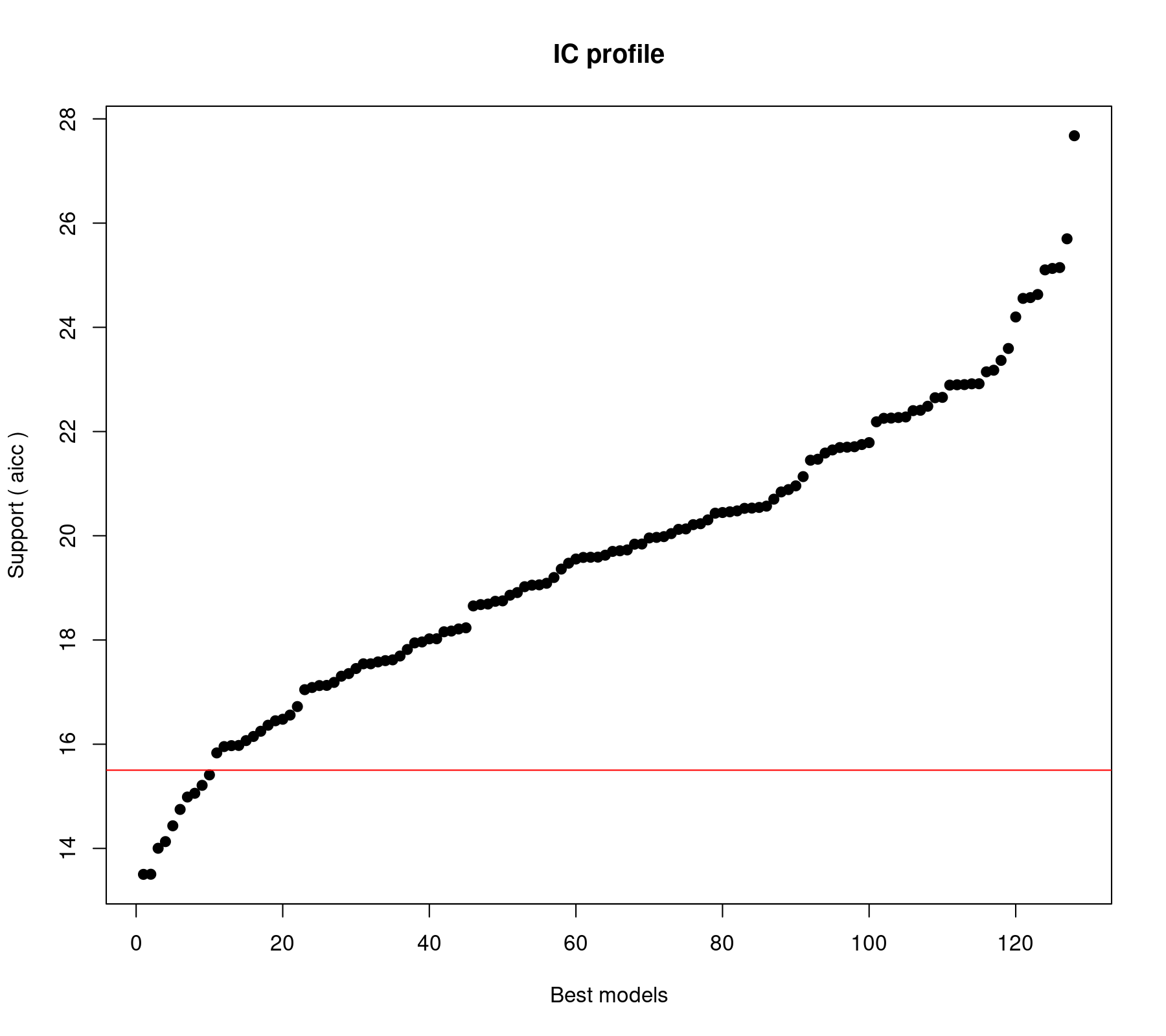
The horizontal red line differentiates between models whose AICc value is less versus more than 2 units away from that of the "best" model (i.e., the model with the lowest AICc). The output above shows that there are 10 such models. Sometimes this is taken as a cutoff, so that models with values more than 2 units away are considered substantially less plausible than those with AICc values closer to that of the best model. However, we should not get too hung up about such (somewhat arbitrary) divisions (and there are critiques of this rule; e.g., Anderson, 2008).
But let's take a look at the top 10 models:
top <- weightable(res)
top <- top[top$aicc <= min(top$aicc) + 2,]
top
                             model     aicc    weights
1                    yi ~ 1 + imag 13.50225 0.06705689
2             yi ~ 1 + imag + meta 13.50451 0.06698091
3         yi ~ 1 + feedback + imag 14.00315 0.05220042
4           yi ~ 1 + length + imag 14.13095 0.04896916
5  yi ~ 1 + feedback + imag + meta 14.43433 0.04207684
6       yi ~ 1 + wic + imag + meta 14.74833 0.03596327
7  yi ~ 1 + feedback + pers + imag 14.98665 0.03192348
8             yi ~ 1 + pers + imag 15.05819 0.03080169
9    yi ~ 1 + length + imag + meta 15.21061 0.02854148
10             yi ~ 1 + wic + imag 15.41073 0.02582384
We see that the "best" model is the one that only includes imag as a moderator. The second best includes imag and meta. And so on. The values under weights are the model weights (also called "Akaike weights"). From an information-theoretic perspective, the Akaike weight for a particular model can be regarded as the probability that the model is the best model (in a Kullback-Leibler sense of minimizing the loss of information when approximating full reality or the real data generating mechanism by a fitted model) out of all of the models considered/fitted. So, while the "best" model has the highest weight/probability, its weight in this example is not substantially larger than that of the second model (and also the third, fourth, and so on). So, we shouldn't be all too certain here that the top model is really the best model in the set. Several models are almost equally plausible (in other examples, one or two models may carry most of the weight, but not here).
So, we could now examine the "best" model with:
summary(res@objects[[1]])
Mixed-Effects Model (k = 41; tau^2 estimator: ML)

  logLik  deviance       AIC       BIC      AICc
 -3.4268   56.9171   12.8536   17.9943   13.5022

tau^2 (estimated amount of residual heterogeneity):     0.0088 (SE = 0.0084)
tau (square root of estimated tau^2 value):             0.0937
I^2 (residual heterogeneity / unaccounted variability): 20.92%
H^2 (unaccounted variability / sampling variability):   1.26
R^2 (amount of heterogeneity accounted for):            66.58%

Test for Residual Heterogeneity:
QE(df = 39) = 57.8357, p-val = 0.0265

Test of Moderators (coefficient 2):
QM(df = 1) = 9.4642, p-val = 0.0021

Model Results:

         estimate      se    zval    pval   ci.lb   ci.ub
intrcpt    0.1439  0.0347  4.1477  <.0001  0.0759  0.2119  ***
imag       0.4437  0.1442  3.0764  0.0021  0.1610  0.7264   **

---
Signif. codes:  0 ‘***’ 0.001 ‘**’ 0.01 ‘*’ 0.05 ‘.’ 0.1 ‘ ’ 1
And here, we see that imag is indeed a significant predictor of the treatment effect (and since it is a dummy variables, it can change the treatment effect from $.1439$ to $.1439 + .4437 = .5876$, which is also practically relevant (for standardized mean differences, some would interpret this as changing a small effect into at least a medium-sized one). However, now I am starting to mix the information-theoretic approach with classical null hypothesis testing, and I will probably go to hell for all eternity if I do so. Also, other models in the candidate set have model probabilities that are almost as large as the one for this model, so why only focus on this one model?
Variable Importance
Instead, it may be better to ask about the relative importance of the various predictors more generally, taking all of the models into consideration. We can obtain a plot of the relative importance of the various model terms with:
plot(res, type="s")
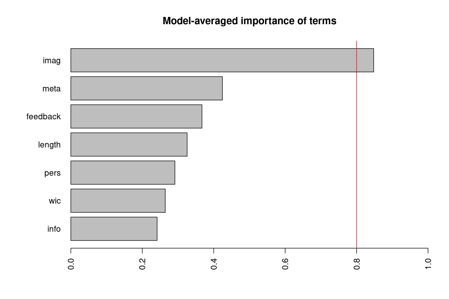
The importance value for a particular predictor is equal to the sum of the weights/probabilities for the models in which the variable appears. So, a variable that shows up in lots of models with large weights will receive a high importance value. In that sense, these values can be regarded as the overall support for each variable across all models in the candidate set. The vertical red line is drawn at 0.8, which is sometimes used as a cutoff to differentiate between important and not so important variables, but this is again a more or less arbitrary division (and a cutoff of 0.5 has also been at times used/suggested).
Multimodel Inference
If we do want to make inferences about the various predictors, we may want to do so not in the context of a single model that is declared to be "best", but across all possible models (taking their relative weights into consideration). Multimodel inference can be used for this purpose. To get the glmulti package to handle rma.uni objects, we must register a getfit method for such objects. The necessary code for this comes with the metafor package, but it first needs to be evaluated with:
eval(metafor:::.glmulti)
Now we can carry out the computations for multimodel inference with:
coef(res, varweighting="Johnson")
The output is not shown, because I don't find it very intuitive. But with a bit of extra code, we can make it more interpretable:
mmi <- as.data.frame(coef(res, varweighting="Johnson"))
mmi <- data.frame(Estimate=mmi$Est, SE=sqrt(mmi$Uncond), Importance=mmi$Importance, row.names=row.names(mmi))
mmi$z <- mmi$Estimate / mmi$SE
mmi$p <- 2*pnorm(abs(mmi$z), lower.tail=FALSE)
names(mmi) <- c("Estimate", "Std. Error", "Importance", "z value", "Pr(>|z|)")
mmi$ci.lb <- mmi[[1]] - qnorm(.975) * mmi[[2]]
mmi$ci.ub <- mmi[[1]] + qnorm(.975) * mmi[[2]]
mmi <- mmi[order(mmi$Importance, decreasing=TRUE), c(1,2,4:7,3)]
round(mmi, 4)
         Estimate Std. Error z value Pr(>|z|)   ci.lb  ci.ub Importance
intrcpt    0.1084     0.1031  1.0514   0.2931 -0.0937 0.3105     1.0000
imag       0.3512     0.2016  1.7414   0.0816 -0.0441 0.7464     0.8478
meta       0.0512     0.0853  0.6003   0.5483 -0.1160 0.2184     0.4244
feedback   0.0366     0.0689  0.5311   0.5954 -0.0985 0.1717     0.3671
length     0.0023     0.0050  0.4527   0.6508 -0.0076 0.0121     0.3255
pers       0.0132     0.0688  0.1925   0.8473 -0.1216 0.1481     0.2913
wic       -0.0170     0.0545 -0.3122   0.7549 -0.1238 0.0897     0.2643
info      -0.0183     0.0799 -0.2286   0.8191 -0.1749 0.1384     0.2416
I rounded the results to 4 digits to make the results easier to interpret. Note that the table again includes the importance values. In addition, we get unconditional estimates of the model coefficients (first column). These are model-averaged parameter estimates, which are weighted averages of the model coefficients across the various models (with weights equal to the model probabilities). These values are called "unconditional" as they are not conditional on any one model (but they are still conditional on the 128 models that we have fitted to these data; but not as conditional as fitting a single model and then making all inferences conditional on that one single model). Moreover, we get estimates of the unconditional standard errors of these model-averaged values.1) These standard errors take two sources of uncertainty into account: (1) uncertainty within a given model (i.e., the standard error of a particular model coefficient shown in the output when fitting a model; as an example, see the output from the "best" model shown earlier) and (2) uncertainty with respect to which model is actually the best approximation to reality (so this source of variability examines how much the size of a model coefficient varies across the set of candidate models). The model-averaged parameter estimates and the unconditional standard errors can be used for multimodel inference, that is, we can compute z-values, p-values, and confidence interval bounds for each coefficient in the usual manner.
Multimodel Predictions
We can also use multimodel methods for computing predicted values and corresponding confidence intervals. Again, we do not want to base our inferences on a single model, but all models in the candidate set. Doing so requires a bit more manual work, as I have not (yet) found a way to use the predict() function from the glmulti package in combination with metafor for this purpose. So, we have to loop through all models, compute the predicted value based on each model, and then compute a weighted average (using the model weights) of the predicted values across all models.
Let's consider an example. Suppose we want to compute the predicted value for studies with a treatment length of 15 weeks that used in-class writing, where feedback was provided, where the writing did not contain informational or personal components, but the writing did contain imaginative components, and prompts for metacognitive reflection were given:
x <- c("length"=15, "wic"=1, "feedback"=1, "info"=0, "pers"=0, "imag"=1, "meta"=1)
Then we can obtain the predicted value for this combination of moderator values based on all 128 models with:
preds <- list()

for (j in 1:res@nbmods) {

   model <- res@objects[[j]]
   vars <- names(coef(model))[-1]

   if (length(vars) == 0) {
      preds[[j]] <- predict(model)
   } else {
      preds[[j]] <- predict(model, newmods=x[vars])
   }

}
The multimodel predicted value is then given by:
weights <- weightable(res)$weights
yhat <- sum(weights * sapply(preds, function(x) x$pred))
round(yhat, 3)
[1] 0.564
We can then compute the corresponding (unconditional) standard error with:
se <- sqrt(sum(weights * sapply(preds, function(x) x$se^2 + (x$pred - yhat)^2)))
Finally, a 95% confidence interval for the predicted average standardized mean difference is then given by:
round(yhat + c(-1,1)*qnorm(.975)*se, 3)
[1] 0.128 1.001
Models with Interactions
One can of course also include models with interactions in the candidate set. However, when doing so, the number of possible models quickly explodes (or even more so than when only considering main effects), especially when fitting all possible models that could be generated based on various combinations of main effects and interaction terms. In the present example, we can figure out how many models that would be with:
glmulti(yi ~ length + wic + feedback + info + pers + imag + meta, data=dat,
        level=2, marginality=TRUE, method="d", fitfunction=rma.glmulti, crit="aicc")
Initialization...
TASK: Diagnostic of candidate set.
Sample size: 41
0 factor(s).
7 covariate(s).
0 f exclusion(s).
0 c exclusion(s).
0 f:f exclusion(s).
0 c:c exclusion(s).
0 f:c exclusion(s).
Size constraints: min =  0 max = -1
Complexity constraints: min =  0 max = -1
Marginality rule.
Your candidate set contains 2350602 models.
[1] 2350602
So, the candidate set would include over two million possible models. Fitting all of these models would not only test our patience (and would be a waste of valuable CPU cycles), it would also be a pointless exercise (even fitting the 128 models above could be critiqued by some as a mindless hunting expedition – although if one does not get too fixated on the best model, but considers all the models in the set as part of a multimodel inference approach, this critique loses some of its force). So, I won't consider this any further in this example.
Using the MuMIn Package
One disadvantage of the glmulti package is that it requires Java to be installed on the computer (so if you install and load the glmulti package and get an error that the rJava package could not be loaded, this is likely to reflect this missing system requirement). As an alternative, we can also use the MuMIn package. So, let's replicate the results we obtained above.
First, we install and load the MuMIn package and then evaluate some code that generates two necessary helper functions we need so that MuMIn and metafor can interact as necessary:
install.packages("MuMIn")
library(MuMIn)
eval(metafor:::.MuMIn)
Next, we fit the full model with:
full <- rma(yi, vi, mods = ~ length + wic + feedback + info + pers + imag + meta,
            data=dat, method="ML")
Now we can fit all 128 models and examine those models whose AICc value is no more than 2 units away from that of the best model with:
res <- dredge(full, trace=2)
subset(res, delta <= 2, recalc.weights=FALSE)
Global model call: rma(yi = yi, vi = vi, mods = ~length + wic + feedback + info +
    pers + imag + meta, data = dat, method = "ML")
---
Model selection table
   (Intrc)   fdbck   imag    lngth    meta    pers      wic df logLik AICc delta weight
3        +         0.4437                                    3 -3.427 13.5  0.00  0.067
19       +         0.4020          0.10880                   4 -2.197 13.5  0.00  0.067
4        + 0.09907 0.4359                                    4 -2.446 14.0  0.50  0.052
11       +         0.4059 0.007695                           4 -2.510 14.1  0.63  0.049
20       + 0.09112 0.3967          0.10140                   5 -1.360 14.4  0.93  0.042
83       +         0.4209          0.12500         -0.09359  5 -1.517 14.7  1.25  0.036
36       + 0.11820 0.3869                  0.08858           5 -1.636 15.0  1.48  0.032
35       +         0.4072                  0.06671           4 -2.974 15.1  1.56  0.031
27       +         0.3812 0.005604 0.09186                   5 -1.748 15.2  1.71  0.029
67       +         0.4608                          -0.05935  4 -3.150 15.4  1.91  0.026
Models ranked by AICc(x)
Note that, by default, subset() recalculates the weights, so they sum to 1 for the models shown. To get the same results as obtained with glmulti, I set recalc.weights=FALSE. If you compare these results to those in object top, you will see that they are same.
Multimodel inference can be done with:
summary(model.avg(res))
Model-averaged coefficients:
(full average)
          Estimate Std. Error z value Pr(>|z|)
intrcpt   0.108404   0.103105   1.051   0.2931
imag      0.351153   0.201648   1.741   0.0816 .
meta      0.051201   0.085290   0.600   0.5483
feedback  0.036604   0.068926   0.531   0.5954
length    0.002272   0.005019   0.453   0.6508
wic      -0.017004   0.054466   0.312   0.7549
pers      0.013244   0.068788   0.193   0.8473
info     -0.018272   0.079911   0.229   0.8191
I have removed some of the output, since this is the part we are most interested in. These are the same results as in object mmi shown earlier.
Finally, the relative importance values for the predictors can be obtained with:
sw(res)
                     imag meta feedback length pers wic  info
Sum of weights:      0.85 0.42 0.37     0.33   0.29 0.26 0.24
N containing models:   64   64   64       64     64   64   64
These are again the same values we obtained earlier.
Other Model Types
The same principle can of course be applied when fitting other types of models, such as those that can be fitted with the rma.mv() or rma.glmm() functions. One just has to write an appropriate rma.glmulti function when using the glmulti package (when using the MuMIn package, one simply applies the dredge() function to the full model). An example illustrating the use of model selection with a fairly complex rma.mv() model can be found here (the example involves only a small number of predictors, but also considers their interaction and also illustrates using parallel processing when using the dredge() function).
For multivariate/multilevel models fitted with the rma.mv() function, one can also consider model selection with respect to the random effects structure. Making this work would require a bit more work. Time permitting, I might write up an example illustrating this at some point in the future.
References
Anderson, D. R. (2008). Model based inference in the life sciences: A primer on evidence. New York: Springer.
Bangert-Drowns, R. L., Hurley, M. M., & Wilkinson, B. (2004). The effects of school-based writing-to-learn interventions on academic achievement: A meta-analysis. Review of Educational Research, 74(1), 29–58.
Burnham, K. P., & Anderson, D. R. (2002). Model selection and multimodel inference: A practical information-theoretic approach (2nd ed.). New York: Springer.
Gurka, M. J. (2006). Selecting the best linear mixed model under REML. American Statistician, 60(1), 19-26.
1)
Above, we used
tips/model_selection_with_glmulti_and_mumin.txt · Last modified: by Wolfgang Viechtbauer