The metafor Package

Journals have different requirements as to how a forest plot should be drawn and the various pieces of information that should be included in the figure. For example, the figure below was extracted from the article by Goldenberg et al. (2021) from the British Medical Journal (see Figure 3).

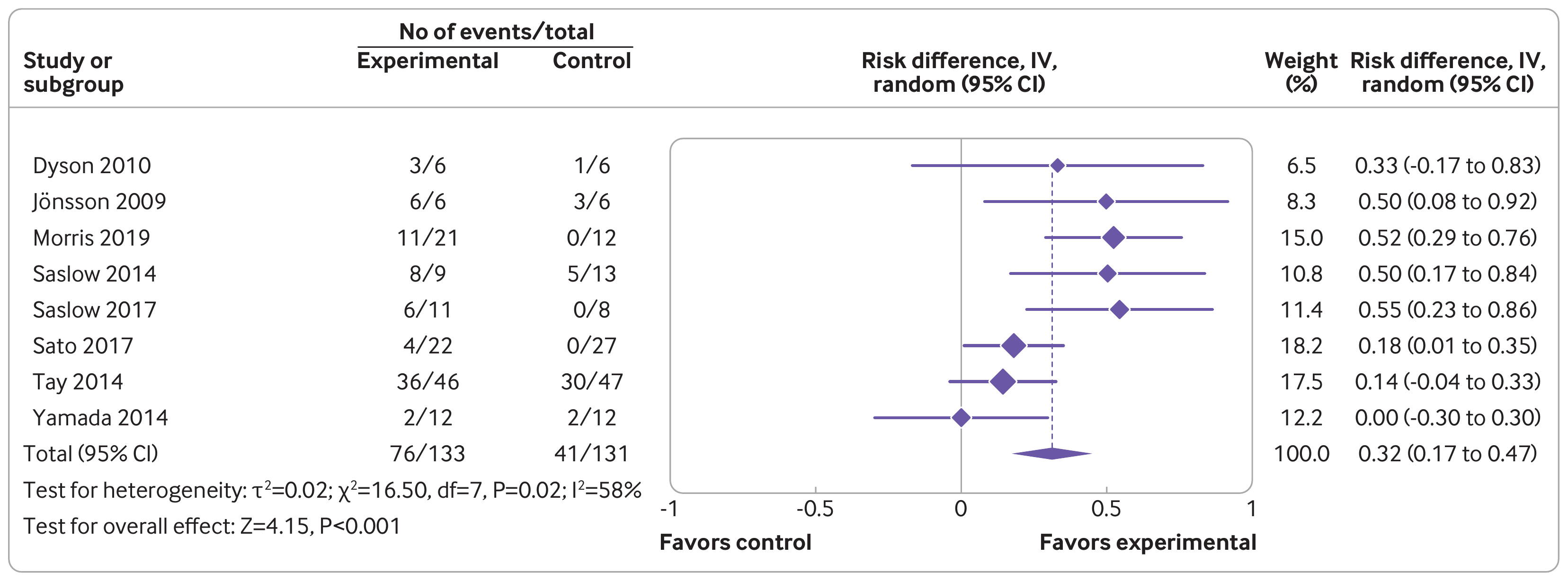
One of the strengths of R is its flexibility when creating figures. The code below shows how the figure can be recreated using a combination of the forest() function from metafor and using functions such as text() and points() to add additional elements to the figure in the same style as done in the article. Note that it takes a bit of work to recreate the figure, although some parts are really optional (the goal here was to recreate the figure as closely as possible, except for a few minor deviations in terms of the alignment of the elements and leaving out the rounded boxes). Also note that one really needs to save the figure to a file for it to look right. The figure below was saved with png(filename="forest_plot_bmj.png", res=315, width=3312, height=1228).¹⁾

### create the dataset (from Goldenberg et al., 2021; http://dx.doi.org/10.1136/bmj.m4743)
dat <- data.frame(author = c("Dyson", "Jönsson", "Morris", "Saslow", "Saslow", "Sato", "Tay", "Yamada"),
                  year   = c(2010, 2009, 2019, 2014, 2017, 2017, 2014, 2014),
                  ai     = c(3, 6, 11, 8, 6, 4, 36, 2),
                  n1i    = c(6, 6, 21, 9, 11, 22, 46, 12),
                  ci     = c(1, 3, 0, 5, 0, 0, 30, 2),
                  n2i    = c(6, 6, 12, 13, 8, 27, 47, 12))
 
### calculate risk differences and corresponding sampling variances (and use
### the 'slab' argument to store study labels as part of the data frame)
dat <- escalc(measure="RD", ai=ai, n1i=n1i, ci=ci, n2i=n2i, data=dat,
              slab=paste(" ", author, year), addyi=FALSE)
dat
 
### fit random-effects model (using the DL estimator)
res <- rma(yi, vi, data=dat, method="DL")
res
 
############################################################################
 
### colors to be used in the plot
colp <- "#6b58a6"
coll <- "#a7a9ac"
 
### total number of studies
k <- nrow(dat)
 
### generate point sizes
psize <- weights(res)
psize <- 1.2 + (psize - min(psize)) / (max(psize) - min(psize))
 
### get the weights and format them as will be used in the forest plot
weights <- fmtx(weights(res), digits=1)
 
### adjust the margins
par(mar=c(2.7,3.2,2.3,1.3), mgp=c(3,0,0), tcl=0.15)
 
### forest plot with extra annotations
sav <- forest(dat$yi, dat$vi, xlim=c(-3.4,2.1), ylim=c(-0.5,k+3), alim=c(-1,1), cex=0.88,
              pch=18, psize=psize, efac=0, refline=NA, lty=c(1,0), xlab="",
              ilab=cbind(paste(dat$ai, "/", dat$n1i), paste(dat$ci, "/", dat$n2i), weights),
              ilab.xpos=c(-1.9,-1.3,1.2), annosym=c(" (", " to ", ")"),
              rowadj=-.07)
 
### add the vertical reference line at 0
segments(0, -1, 0, k+1.6, col=coll)
 
### add the vertical reference line at the pooled estimate
segments(coef(res), 0, coef(res), k, col=colp, lty="33", lwd=0.8)
 
### redraw the CI lines and points in the chosen color
segments(summary(dat)$ci.lb, k:1, summary(dat)$ci.ub, k:1, col=colp, lwd=1.5)
points(dat$yi, k:1, pch=18, cex=psize*1.15, col="white")
points(dat$yi, k:1, pch=18, cex=psize, col=colp)
 
### add the summary polygon
addpoly(res, row=0, mlab="Total (95% CI)", efac=2, col=colp, border=colp)
 
### add the horizontal line at the top
abline(h=k+1.6, col=coll)
 
### redraw the x-axis in the chosen color
axis(side=1, at=seq(-1,1,by=0.5), col=coll, labels=FALSE)
 
### now we add a bunch of text; since some of the text falls outside of the
### plot region, we set xpd=NA so nothing gets clipped
par(xpd=NA)
 
### adjust cex as used in the forest plot and use a bold font
par(cex=sav$cex, font=2)
 
### add headings
text(sav$xlim[1], k+2.5, pos=4, "Study or\nsubgroup")
text(sav$ilab.xpos[1:2], k+2.3, c("Experimental","Control"))
text(mean(sav$ilab.xpos[1:2]), k+3.4, "No of events / total")
text(0, k+2.7, "Risk difference, IV,\nrandom (95% CI)")
segments(sav$ilab.xpos[1]-0.22, k+2.8, sav$ilab.xpos[2]+0.13, k+2.8)
text(c(sav$ilab.xpos[3],sav$xlim[2]-0.35), k+2.7, c("Weight\n(%)","Risk difference, IV,\nrandom (95% CI)"))
 
### add 'Favours control'/'Favours experimental' text below the x-axis
text(c(-1,1), -2.5, c("Favors control","Favors experimental"), pos=c(4,2), offset=-0.3)
 
### use a non-bold font for the rest of the text
par(cex=sav$cex, font=1)
 
### add the 100.0 for the sum of the weights
text(sav$ilab.xpos[3], 0, "100.0")
 
### add the column totals for the counts and sample sizes
text(sav$ilab.xpos[1:2], 0, c(paste(sum(dat$ai), "/", sum(dat$n1i)), paste(sum(dat$ci), "/", sum(dat$n2i))))
 
### add text with heterogeneity statistics
text(sav$xlim[1], -1, pos=4, bquote(paste("Test for heterogeneity: ",
   tau^2, "=", .(fmtx(res$tau2, digits=2)), "; ",
   chi^2, "=", .(fmtx(res$QE, digits=2)),
   ", df=", .(res$k - res$p), ", ",
   .(fmtp(res$QEp, digits=2, pname="P", add0=TRUE, equal=TRUE)), "; ",
   I^2, "=", .(round(res$I2)), "%")))
 
### add text for test of overall effect
text(sav$xlim[1], -2, pos=4, bquote(paste("Test for overall effect: ",
   "Z=", .(fmtx(res$zval, digits=2)), ", ",
   .(fmtp(res$pval, digits=3, pname="P", add0=TRUE, equal=TRUE)))))