llplot() function would have omitted this study from the plot by default. With drop00=FALSE, we can also see the (flat) likelihood for this study.The paper by van Houwelingen et al. (1993) is an early (and unfortunately often overlooked) paper on meta-analytic methods for 2×2 table data that describes a variety of rather sophisticated models and methods, including the equal- and random-effects conditional logistic models, a nonparametric mixture model based on Laird (1978), and the bivariate binomial-normal model. The models and methods are illustrated with data from 27 studies examining the effectiveness of histamine H2 antagonists (cimetidine or ranitidine) in treating patients with acute upper gastrointestinal hemorrhage. The dataset can be loaded with:
library(metafor)
dat <- dat.collins1985a
dat
(I copy the dataset into dat, which is a bit shorter and therefore easier to type further below). Variables nti and nci in this dataset indicate the number of patients in the treatment and control groups, respectively, while b.xti and b.xci indicate the number of patients with persistent or recurrent bleedings in the respective groups.
No information about this outcome was available for 2 trials, so the results below are based on the remaining 25 trials. Also, note that van Houwelingen et al. (1993) analyze the log odds ratios of persistent or recurrent bleedings in the control group versus the treatment group, so that positive values indicate a lower risk in the treatment group and hence a positive treatment effect.
Among the models considered by the authors is the equal-effects conditional logistic model (described as a "likelihood based Mantel-Haenszel-type procedure" in the article). The model results from conditioning on the total number of cases within each study, leading to the non-central hypergeometric distribution for the 2×2 tables. Figure 2 in the paper (p. 2277) shows the likelihoods of the log odds ratios based on the non-central hypergeometric distributions for the individual studies. An analogous figure can be produced with:
llplot(measure="OR", ai=b.xci, n1i=nci, ci=b.xti, n2i=nti, data=dat,
       xlim=c(-4,4), lwd=2.0, col="black", refline=NA, drop00=FALSE)
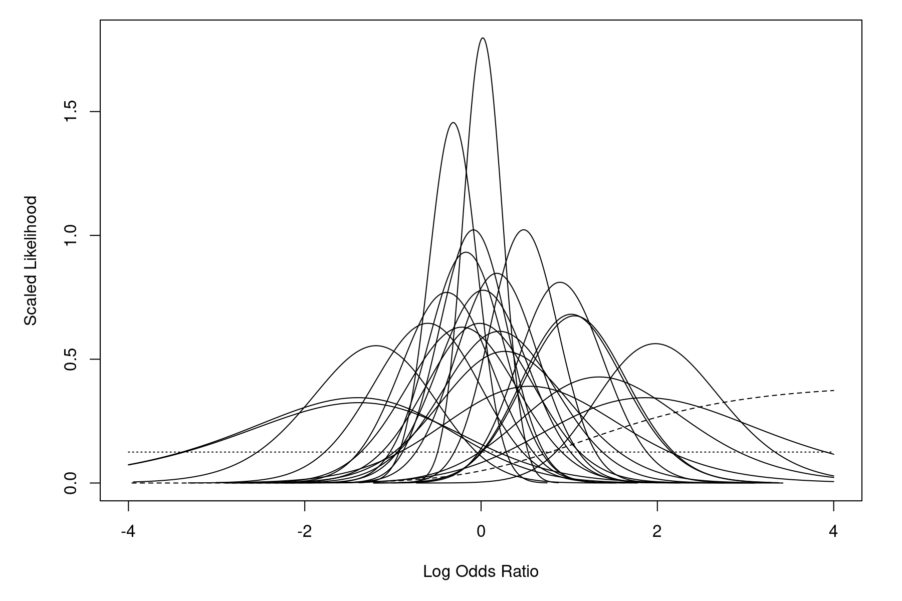
One study (number 10) has a single zero cell (none of the patients in the treatment group experienced persistent or recurrent bleedings), which implies that the MLE of the odds ratio is infinite. The dashed line in the figure corresponds to this study. Also, one study (number 14) has two zero cells (none of the patients in the entire study experienced persistent or recurrent bleedings), which implies a flat likelihood for the odds ratio. The dotted line in the figure corresponds to this study.1) However, for most studies, the likelihood is concentrated within the range $-1$ to $1$. Hence, the MLE of the log odds ratio should also fall somewhere within this range.
The results from a corresponding equal-effects model can be obtained with:
res <- rma.glmm(measure="OR", ai=b.xci, n1i=nci, ci=b.xti, n2i=nti,
                data=dat, model="CM.EL", method="EE")
summary(res, digits=2)
Equal-Effects Model (k = 24)
Model Type: Conditional Model with Exact Likelihood

  logLik  deviance       AIC       BIC      AICc
  -53.68     40.34    109.36    110.54    109.54

Tests for Heterogeneity:
Wld(df = 23) = 32.52, p-val = 0.09
LRT(df = 23) = 40.34, p-val = 0.01

Model Results:

estimate    se  zval  pval  ci.lb  ci.ub
    0.12  0.10  1.22  0.22  -0.07   0.32

---
Signif. codes:  0 '***' 0.001 '**' 0.01 '*' 0.05 '.' 0.1 ' ' 1
These results match what is reported on page 2275. In particular, the log odds ratio is estimated to be $\hat{\theta} = 0.12$ (with 95% confidence interval: $-0.07$ to $0.32$). The log likelihood for this model is $ll = -53.68$.
Note that this method will give very similar results as the well-known Mantel-Haenszel method, which is also in essence based on a conditional hypergeometric model. We can compare the results above to those obtained with the Mantel-Haenszel method below.
rma.mh(measure="OR", ai=b.xci, n1i=nci, ci=b.xti, n2i=nti, data=dat, digits=2)
Equal-Effects Model (k = 25)

I^2 (total heterogeneity / total variability):  33.94%
H^2 (total variability / sampling variability): 1.51

Test for Heterogeneity:
Q(df = 23) = 34.82, p-val = 0.05

Model Results (log scale):

estimate    se  zval  pval  ci.lb  ci.ub
    0.12  0.10  1.22  0.22  -0.07   0.32

Model Results (OR scale):

estimate  ci.lb  ci.ub
    1.13   0.93   1.37

Cochran-Mantel-Haenszel Test:    CMH =  1.37, df = 1,  p-val = 0.24
Tarone's Test for Heterogeneity: X^2 = 38.71, df = 23, p-val = 0.02
The model results are identical when rounded to two decimal places.
The corresponding random-effects model (described as a "random effects extension of the Mantel-Haenszel procedure" in the paper) can be obtained by assuming a normal distribution for the true log odds ratios of the individual studies. We then obtain a random-effects conditional logistic model, which can be fitted with:2)
res <- rma.glmm(measure="OR", ai=b.xci, n1i=nci, ci=b.xti, n2i=nti,
                data=dat, model="CM.EL", method="ML")
summary(res, digits=2)
Random-Effects Model (k = 24; tau^2 estimator: ML)
Model Type: Conditional Model with Exact Likelihood

  logLik  deviance       AIC       BIC      AICc
  -52.99     38.96    109.98    112.34    110.55

tau^2 (estimated amount of total heterogeneity): 0.12 (SE = 0.14)
tau (square root of estimated tau^2 value):      0.35
I^2 (total heterogeneity / total variability):   30.86%
H^2 (total variability / sampling variability):  1.45

Tests for Heterogeneity:
Wld(df = 23) = 32.52, p-val = 0.09
LRT(df = 23) = 40.34, p-val = 0.01

Model Results:

estimate    se  zval  pval  ci.lb  ci.ub
    0.17  0.14  1.28  0.20  -0.09   0.44

---
Signif. codes:  0 '***' 0.001 '**' 0.01 '*' 0.05 '.' 0.1 ' ' 1
These results match what is reported on page 2277. In particular, the estimated average log odds ratio is $\hat{\mu} = 0.17$ (with 95% confidence interval: $-0.09$ to $0.44$),3) while the estimated amount of heterogeneity is $\hat{\tau}^2 = .35^2$. The log likelihood for this model is $ll = -52.99$.
Instead of assuming normally distributed random effects, van Houwelingen et al. (1993) also discuss the use of a nonparametric mixture model based on Laird (1978). The components of such a non-parametric mixture can be estimated by means of the CAMAN package in two steps. First, we must estimate the individual log odds ratios and corresponding sampling variances, which can be done with:
dat <- escalc(measure="OR", ai=b.xci, n1i=nci, ci=b.xti, n2i=nti, data=dat)
dat <- dat[!is.na(dat$yi),]
Note that we must also manually remove rows where the log odds ratios cannot be computed. Then we can fit the nonparametric mixture model with:
library(CAMAN)
res <- mixalg(obs="yi", var="vi", data=dat)
res
Computer Assisted Mixture Analysis:

Data consists of 25 observations (rows).
The Mixture Analysis identified 2 components of a gaussian distribution:

DETAILS:
          p         mean
1 0.8183766 -0.008554017
2 0.1816234  1.036847813

Log-Likelihood: -28.87813     BIC: 67.41289
As in the article, we obtain a two-point distribution, with one component close to 0 (i.e., $OR \approx 1$) and one component around 1 (i.e., $OR \approx 2.7$). However, the exact component values and corresponding probabilities are slightly different (van Houwelingen et al. base their mixture model directly on the non-central hypergeometric distribution, while the model fitted above approximates the sampling distributions of the observed log odds ratios with normal distributions).
Collins, R., & Langman, M. (1985). Treatment with histamine H2 antagonists in acute upper gastrointestinal hemorrhage: Implications of randomized trials. New England Journal of Medicine, 313(11), 660–666.
van Houwelingen, H. C., Zwinderman, K. H., & Stijnen, T. (1993). A bivariate approach to meta-analysis. Statistics in Medicine, 12(24), 2273–2284.
Laird, N. M. (1978). Nonparametric maximum likelihood estimation of a mixing distribution. Journal of the American Statistical Association, 73(364), 805–811.
llplot() function would have omitted this study from the plot by default. With drop00=FALSE, we can also see the (flat) likelihood for this study.